方案详情文
智能文字提取功能测试中
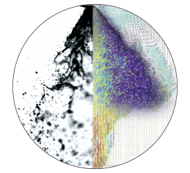
1This draft was prepared using the LaTeX style file belonging to the Journal of Fluid Mechanics M. Soleimani nia, B. Marwell, P. Oshkai and N. Djilali2 t Email address for correspondence: majids@uvic.ca Measurements of Flow Velocity and ScalarConcentration in TurbulentMulti-component Jets: Asymmetry andBuoyancy Effects Majid Soleimani nialt, Brian Maxwell2, Peter Oshkail and NedDjilali Department of Mechanical Engineering and Institute for Integrated Energy Systems,University of Victoria, PO Box 1700 STN CSC, Victoria, BC,V8W 2Y2, Canada "Department of Mechanical and Aerospace Engineering, Case Western Reserve University,10900 Euclid Avenue, Glennan 418, Cleveland Ohio, 44106, USA (Received xx; revised xx; accepted xx) Buoyancy effects and nozzle geometry can have a significant impact on turbulent jetdispersion. This work was motivated by applications involving hydrogen. Using heliumas an experimental proxy, buoyant horizontal jets issuing from a round orifice on the sidewall of a circular tube were analysed experimentally using particle image velocimetry(PIV) and planar laser-induced fluorescence (PLIF) techniques simultaneously to provideinstantaneous and time-averaged flow fields of velocity and concentration. Effects ofbuoyancy and asymmetry on the resulting flow structure were studied over a rangeof Reynolds numbers and gas densities. Significant differences were found between thecentreline trajectory, spreading rate, and velocity decay of conventional horizontal roundaxisymmetric jets issuing through flat plates and the pipeline leak-representative jetscAsonsidered in the present study. The realistic pipeline jets were always asymmetric andfound to deflect about the jet axis in the near field. In the far field, it was found that therealistic pipeline leak geometry causes buoyancy effects to dominate much sooner thanexpected compared to horizontal round jets issuing through flat plates. 1. Introduction Hydrogen, a carbon-free energy carrier, is currently viewed as a clean alternative totraditional hydrocarbon-based fuels for transportation and energy storage applications. Itcan burn or react with almost no pollution or green house gas emissions, and is commonlyused in electrochemical fuel cells to power vehicle and electrical devices. It is also usedin an increasing number ofpower-to-gas systems to blend in the natural gas pipelinenetwork. Despite these benefits, previous studies have shown that hydrogen jets resultingfrom an accidental leak are easily ignitable(Veser et al.2011), owing to a wide range ofpossible ignition limits (between 4%-75% by volume)i Lewis & von Elbe1961). There e,modern safety standards for hydrogen storage infrastructure must be assured beforewidespread public use of hydrogen can become possible. As a result, fundamental insightinto the physics of hydrogen dispersion into ambient air from realistic flow geometries,such as small pipelines, is necessary to properly predict flow structures and flammabilityenvelope associated with hydrogen outflow from accidental leaks. Also, owing to the lowmolecular weight of hydrogen, buoyancy can significantly influence the development of the jet dispersion during a release scenario. In the current investigation, we attempt toquantify the dispersion and release trajectories of horizontal buoyant jets experimentally,as they emerge from a realistic pipeline geometry, using state-of-the-art experimentalimaging techniques. In the last two decades, due to the rapid development of the hydrogen economy and useof hydrogen technologies, several experimental and numerical studieslChernyavsky et al.2011:Houf & Scheferl2008Schefer et al2008aXiao et al.l22011)have investigatedsmall-i-scale unintendedhydrogen rround jet releasein ambient air, while othersEkotolet al.2012;可Houf et al..2013,2010EHajji et al.2015lstudied different accidental hydrogendispersion scenarios in enclosed and open spaces. There has also been extensive workdone to describe the evolution of axisymmetric round turbulent jets in terms of self-similarity correlations, obtained from statistical analysis from both experimentsLipari& Stansby 2011; Ball et al. 2012and simulations(M. Kaushik2015). In addition, someinvestigations(Su et al2010) have quantified the buoyancy effects on vertical round jets,while othersRodil1982Carazzo et al.2006)have provided a quantitative study intothe buoyancy effects on both turbulent buoyant/pure jets and plumes with analyzing ofall available experimental data. Even though jets and plumes both have different statesof partial or local self-similarity(George1989), their global evolutions in the far fieldtends toward complete self-similarity through a universal route even in the presence ofbuoyancy. Large-scale structures of turbulence drive the evolution of the self-similarityprofile, and buoyancy has an effect in exciting the coherent turbulent structures; thiseffect is more evident in the evolution of plumes into self-similarly much sooner owing tobuoyancy driven turbulence in the near field(Carazzo et al.2006). Horizontal buoyantjets, however, have been much less studied. In general, increasing effects of buoyancy werefound to correlate inversely to the Froude number in axisymmetry horizontal buoyantietsAsh2012) Previous measurements on axisymmetric round hydrogen jetslSchefer et al.20086,a)revealed that, hydrogen jets show the same behavior to jets of helium(Panchapakesan& Lumley1993), propane and other hydrocarbon fuels(Richards&Pitts1993). Inparticular, the intensity of centreline velocity fluctuations are similar between the jetand plume regions. In contrast, mass fraction fluctuation intensities increased from aconstant asymptotic value of about 0.23 in the jet region to 0.33-0.37 in the plume region(Panchapakesan & Lumley71993;Schefer et al.2008a). It has also been well establishedthat the mass fraction fluctuation intensities along the centerline and radial variations arealso independent of initial density differences between ambient and jet fluids, and collapseonto the same curves, different curves in jet and plume regions, when plotted against theappropriate similarity variablesPanchapakesan & Lumley1993chefer et al.2008aPittsl1991a). It is noteworthy that all aforementioned studies, as well as related previous investi-gations on jets or plumes, have been limited to leaks through flat surfaces, where thedirection of the jet mean flow was aligned with the flow origin. In reality, however, flowpatterns and dispersion of accidental gas leaks would not be limited to flows throughflat surfaces, and leaks through cracks in the side walls of circular pipes should alsoreceive attention. To address this, a recent study was investigated for vertical buoyantjet evolutions through round holes from curved surfaces, numerically and experimentallySoleimani nia et al.2018Soleimani nia et al.2017 Maxwell et al.2017). Through thisrecent work, significant discrepancies were found between the evolution of axisymmetricround sharp-edged Orifice Plate (OP) jets through flat surfaces and those originatingfrom curved surfaces. Most notably,jet deflection from the vertical axis, and asymmetric FIGURE 1. a) Schematic of the experimental layout. b) Illustration of horizontal 3D jet flowmeasurement area (red inset in part a). dispersion patterns are always observed in realistic situations. To our knowledge, however,the horizontal jet dispersion from curved surfaces has not yet been investigated. To investigate the effects of asymmetry and buoyancy on the evolution of horizontaljets issuing from realistic pipeline geometries, jet release experiments were conductedwith air and helium, where flow patterns and dispersion of gas through a curved surfaceoriginating from a source whose original velocity components were nearly perpendicularto the direction of the ensuing jets. From now on, this jet configuration is referred as a3D jet. A round hole as one of possible crack geometries, was considered in this study,although another possibility might include thin cracks around the tube or the faulty tubefittingslverson et al.2015), which is not considered here. The horizontal 3D jets werereleased through a 2 mm diameter round hole in the side of a round tube (closed at oneend), with an outer diameter of 6.36 mm and 0.82 mm wall thickness. The outer-scaleflow Reynolds numbers (Res), based on the orifice diameter, and Mach numbers (Ma)of the jets ranged from 19,000 to 51,500 and 0.4 to 1.2, respectively. However, it is notedthat for hydrogen jets of equivalent momentum flux, the expected Mach number andReynolds number would be 1.5 and 55,915, respectively. At these conditions, hydrogen isexpected to behave very similar to the helium jets considered hereSoleimani nia et al.2018)). These realistic jets were also compared to axisymmetric leaks through flat surfacesaccordingly. Particle imaging velocimetry (PIV) and planar laser-induced fluorescence(PLIF)were used to measure high-resolution instantaneous velocity and concentrationfields, respectively. The purpose of this investigation was to identify and characterizedepartures from standard axisymmetric jet conditions, and to highlight the buoyancyeffect and asymmetric nature of the 3D jets, which ensued from a practical geometryarrangement. It should be noted that, the effect of pipe wall thickness of the crackgeometry has not yet been investigated. 2. Experimental system and techniques 2.1. Flow facility FigureTa, provides a schematic of the experimental setup used for this study. While,Figure 1b, illustrates the jet flow evolution from the tube orifice considered. To capturethe three-dimensionality of the jet, measurements were obtained on two different two-dimensional planes (denoted ac-z and a-y), as indicated, for both air and helium. Alsoshown in the figure is the jet centreline, which acts as a reference from which measure-ments are later obtained in the s-z plane. Owing to potential deviation of the jet fromthe orifice axis (a-axis), the jet centreline tangent and normal lines are shown as s andn coordinates in the figure, respectively. Jet Orientation Q (uj) Pj Vj Ma Fr Re ,Type [L/min] m/s] 1 [Kg/m²] [m²/s] [N/m] Air H, 3D 15 147.5 1.17 1.54×10 -5 50.9 0.43 - 19,000 Air V, 3D 15 147.5 1.17 1.54×10 -5 50.9 0.43 19,000 Air V, OP 15 127.6 1.17 1.54x10 -5 38.1 0.37 16,500 He H, 3D 35 399.5 0.165 1.21×10~ -4 51.3 1.2 1.34×10° 51,500 He V,3D 35 399.7 0.165 1.21×10⁻⁴ 51.4 1.2 1.34×10° 51,500 He V, OP 35 341.9 0.165 1.21 ×10⁻⁴ 38.3 1 9.8×10° 44,200 TABLE 1. Flow properties The experiments were conducted within a controlled stagnant environment, at roomtemperature and pressure (T~22°,', po ~ 100 kPa). Flow controllers (Bronkhorst,EL-FLOW series) were used to control mass flow rates of dry air and pure scientificgrade helium to the system, with a high accuracy (standard ±0.5% of reading plus±0.1% full scale) and precision (within 0.2% of the reading). Di-Ethyl-Hexyl-Sebacate(DEHS) tracer particles were used in PIV measurements, while acetone vapour used asfluorescent tracers for the PLIF experiments. After the test gas was mixed and seededwith the PIV and PLIF tracers,the flow entered the test section of the tube. Isothermaland isobaric conditions were ensured in all measurements. Further specific details can befound inSoleimani nia et al.2018). The orifice, through which the gas dispersed,had adiameter of D = 2 mm and was located sufficiently downstream along the tube lengthto ensure fully developed flow within the tube at the orifice location. Within the tube,flow controllers were used to ensure fully developed subsonic and turbulent flow insidethe tube. In order to compare the behaviour of both test gases, for each experimental setup,the averaged momentum flux (M) at the jet exit was estimated and matched for all testcases. This matching was achieved iteratively, by varying the volumetric flow rate (Q) inthe system. Here, M was calculated by first obtaining the time-averaged jet exit velocityfrom two-dimensional PIV measurements. The two-dimensional momentum flux, in unitsof [N/m], was then calculated from where the subscript ‘j’refers to the conditions at the nozzle, the angle brackets ‘)’ refer to a time-averaged quantity, and also p and r refer to density and radius,respectively. Table1shows the flow properties used in this study, for the horizontal3D jet configurations, as well as vertical 3D and OP jets used for comparison(Soleimaninia et al.ll2018); H and Vrefer to horizontal and vertical orientations, respectively. In allcases, the jets were characterized by the outer-scale Reynolds number, Re=(uj)8/voo,where, v。 is the ambient fluid kinematic viscosity and 8 is the width of the mean axialvelocity profile, evaluated from limits of 5% of the centreline velocity at x ~0. 2.2. Measurement techniques Particle imaging velocimetry (PIV) was used to capture the two-dimensional velocityflow field information. A dual-head Nd: YAG pulsed laser (New Wave’s SOLO III 15HZ) was used to illuminate a two-dimensional cross-section of the flow, which was seededwith Di-Ethyl-Hexyl-Sebacate (DEHS), with a typical diameter of less than 1 um, to act FIGURE 2. Instantaneous a) velocity and b) molar concentration fields obtained from Helium3D jet in c-z plane from two individual imaging windows stitched together. as a tracer particle. The light sheet had an approximate height of 5 cm and thicknessof 1 mm. The field of view of the camera (PIV CCD) was a 40x30 mm’ window withan approximate pixel size of 6.5 um in physical space. Following the procedure of Sul& Clemens(2003, we estimate this resolution to be comparable to the finest scales ofthe flow, with respect to the Nyquist criterion. Each pair of images were then processedusing LaVision DaVis 8.4 software to calculate the global instantaneous flow velocity field.Following the PIV uncertainty propagation methodSciacchitano & Wieneke2016),.weestimated conservative uncertainty values of 3% and 6% in the time-averaged velocityand Reynolds shear stress profiles, respectively. To measure the gas concentration, we applied planar laser-induced fluorescence (PLIF).To simultaneously apply PLIF, the flow was also seeded with acetone vapour at consistentrate of ~ 10% by volume. A Pulsed Nd: YAG laser (Spectra-Physics INDI-40-10-HG)was used in order to excite the acetone molecules in a light sheet with an approximateheight of 5 cm and a thickness of 350 um, which was then recorded with a PLIF CCDcamera. The camera field of view for all cases corresponded to a 38×28 mm windowwith an approximate pixel size of 6.5 um. The images were taken at a frequency of 5 Hzand then processed using LaVision DaVis 8.4 software. Following correcting for errorsassociated with background noise, fluctuations in cross-sectional laser beam intensity,and laser energy per pulse deviations, one can assume the remaining non-uniformityof the scalar field is due to signal to noise ratio (S/N). The error in the S/N can beestimated from the standard deviation ofthis ratio in an uniform low signal region of theflow field. Based on this data, and uncertainty propagation method, we estimated theuncertainty in the time-averaged and variances of concentration field to be conservativevalues of 4% and 7%, respectively. For each experimental case, a total of 500 images wereacquired to determine the time-averaged molar concentration,(X), and variances, Xfields. Further details of the experimental procedure can be found in(Soleimani nia et al.2018). Finally, to retain the spatial resolution of the flow field, the full measurement regionis covered by two individual imaging windows with at least a 20% overlap between eachwindow. Figure 2 shows examples of the instantaneous velocity and concentration fields,for the helium 3D jet in the s-z plane. It should be noted that the flow fields wereconstructed from two different experiments, where individual imaging windows have beenstitched together. Distances reported here have been normalized such that where D, the diameter of the orifice, is taken as the reference length scale. FIGURE 3. Time-averaged velocity and molar concentration contours from round jet on sideof tube (3D jet) for air and helium, obtained from a) velocity contours in sc-z plane, b) molarconcentration contours in a-z plane, c) velocity contours in c-y plane and d) molar concentrationcontours in x-y plane. 3. Results 3.1.T1ime-averaged flow fields The time-averaged velocity and molar concentration contours, obtained in both thexc-z and a-y planes for all of the 3D jet experiments conducted here, are shown inFig.3For both experiments, significantly larger jet spreading was observed in the s-zplanes compared to the a-y plane. Clearly, the flow structure was asymmetric in bothexperiments. The jets were also found to deviate significantly from the horizontal c-axis,for both gases in the x-z plane. In this plane, near the potential-core region, there wasalso more jet spreading on the lower side of the jet compared to the top side. In the-y planes of both gases, there were two high-velocity peaks (saddle-back behaviour), aty±0.5D, on each side of the s-axis, with a much shorter potential-core length (≈2D)compared to the s-z plane. This saddle-back behaviour was previously found to originatefrom a velocity deficit region which forms inside the orifice due to flow separation as thegas inside the tube encountered the edge of the orifice (Soleimani nia et al.2018). Also, 14 FIGURE 44. Jet centre-lines taken along the location of maximum velocity magnitudes(/u)|max(z)) in s-z plane from measurements. Also shown for comparison are vertical 3D& OP jets(Soleimani nia et al.2018and horizontal round OP jets experimentsAsh2012. there was a shorter potential-core length observed for helium (≈3D), compared to air(≈5D), as observed in the velocity contours of the x-z planes. In general, the concentration profiles were qualitatively similar to the velocity profilespresented in Fig.[3. with two exceptions. First, the concentration core lengths in bothplanes were found to be shorter than the velocity potential cores. The concentrationcore lengths were approximately ≈ 4D in the c-z plane for both gases, and ≈2D and≈1D,for air and helium, respectively in the s-y plane. Also, much higher concentrationlevels, with higher spreading rates, were observed for helium in the far field compared toair. This observation can be attributed to a low Schmidt number (Sc <1), where massdiffusion rates are higher than momentum diffusion rates. 3.2. The jet centreline trajectory In Fig.4the jet centreline trajectories, determined in the xc-z plane, are presented forall cases. Here, the trajectories were determined by the maximum velocity magnitude,u)max(c), locations. Also shown for comparison are the jet centreline trajectoriesobtained from previous vertical 3D jet experiments(Soleimani nia et al.2018),andfrom horizontal sharp-edged orifice flat-plate (OP) helium jet measurementsAshl2012).In order to determine the effect of buoyancy on the horizontal jets, lines of best fit,using linear regression to power law expressions, were obtained for the far field (beyondx ≥10D), and are also shown in Fig. In general, the jet trajectory for the verticaland horizontal air jets were found to be described by a nearly linear relation (i.e. powerlaw exponent ~ 1). The horizontal helium jet, however, was found to have a powerlaw exponent ~ 1.3. Upon extrapolating these relations to the far field, beyond theexperimental data collected, it became clear that buoyancy of the helium jet causedsignificant deflection from the horizontal axis, despite the high Froude number (Fr=1.34 ×10). It should be noted that for horizontal flat-plate OP helium jets, with acomparable Froude number (Fr =1×10⁶), such buoyancy effects were not observedAsh2012. FIGURE 5. a) Inverse time-averaged velocity decay and b) jet velocity widths (2Lu(1/2)) obtainedalong the (u)max(r) centrelines, in xc-zplane from measurements.Note, n-coordinate refersto lines which are normal to the centreline, and coplanar with the x-z plane (see the coordinatesystem in Fig.1 b). Also shown, for comparison are axisymmetric round jet correlationslWitze1974), and vertical 3D & OpJjets, horizontal round OP'jets and round pipe jet experiments(Soleimani nia et al.2018:Ash2012:EHussein et al.1994:Amielh et al.1996 3.3. Velocity decay and jet spreading rates Fig.5a shows the inverse time-averaged velocity decay ((uj)/(uc)) along the jetcentrelines (s-coordinate illustrated in Fig.1b) for all experiments. Here, the subscript‘C'refers to the conditions at the jet centreline, while the subscript‘’refers to thejet exit condition. Also shown, for comparison, are velocity decay correlationsWitzel1974)for compressible subsonic and supersonic axisymmetric round jets, alongwithvelocity decay rates obtained from vertical 3D and OP jet experimentsSoleimani nialet al.2018), and horizontal OP helium jet measurements(Ash2012).Upon comparisonto the Witze correlations(Witze1974), the air and helium OP jet experiments werefound to reproduce well the expected velocity decay rate, with helium jet decaying fasterthan the air jet. On the other hand, the decay rates observed in the experimental 3Djets were much faster compared to the axisymmetric jets. In general, upon comparisonbetween horizontal and vertical 3D jets, buoyancy was not found to significantly affectthe velocity decay rates. In the x-z plane, Figure5b presents the jet velocity widths (2Lu(1/2)), that havebeen obtained by determining the locations where (u)|=0.5(u)max(c) along lineswhich were orthogonal to the jet-centrelines. These orthogonal lines have been indicatedpreviously as coordinate ‘n’in Fig. b. For the 3D jets, in all cases, a slight contraction inthe jet widths has been observed from 1D
-
1/22
-
2/22
还剩20页未读,是否继续阅读?
继续免费阅读全文产品配置单

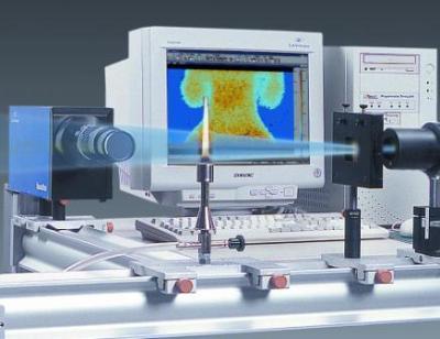
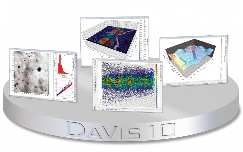
北京欧兰科技发展有限公司为您提供《湍流多组分喷流中流速和标量浓度检测方案(激光粒度仪)》,该方案主要用于其他中流速和标量浓度检测,参考标准《暂无》,《湍流多组分喷流中流速和标量浓度检测方案(激光粒度仪)》用到的仪器有LaVision SprayMaster 喷雾成像测量系统、LaVision IRO 图像增强器、德国LaVision PIV/PLIF粒子成像测速场仪、PLIF平面激光诱导荧光火焰燃烧检测系统、LaVision DaVis 智能成像软件平台。
我要纠错
推荐专场
CCD相机/影像CCD
更多


相关方案
 咨询
咨询