

方案详情文
智能文字提取功能测试中
CHAPTER 1..1INTRODUCTION2 CHAPTER 1...JINTRODUCTION3 ENSTROPHY TRANSPORT IN PREMIXED SWIRL FLAMES by Askar Kazbekoy A thesis submitted in conformity with the requirementsfor the degree of Master of Applied ScienceUniversity of Toronto Institute for Aerospace StudiesUniversity of Toronto Copyright 2018 by Askar Kazbekov Abstract Enstrophy Transport in Premixed Swirl Flames Askar KazbekovMaster of Applied Science University of Toronto Institute for Aerospace StudiesUniversity of Toronto 2018 Reynolds-averaged enstrophy transport budgets are measured in turbulent swirl flames usingmicro-tomographic particle image velocimetry (u-TPIV) and CH2O planar laser induced flu-orescence (PLIF) across Ka =11-45. The combined contributions of baroclinic torque anddissipation to enstrophy transport are evaluated by subtracting the vortex-stretching anddilatation terms from the Lagrangian derivatives. Enstrophy production through baroclinictorque dominated over dissipation towards the product sides of the flame brushes. Enstro-phy budgets, conditioned on mean progress-variable and spatial coordinates,have shownthat the magnitude of baroclinic torque increases with bulk flow velocity. A conservativeestimate of the relative significance of baroclinic torque to vortex-stretching was found to beconstant. In contrast to DNS of flames in HIT, the significance of baroclinic torque relativeto vortex-stretching remained constant with bulk flow velocity. The observed flame-scale tur-bulence generation towards the combustion products has implications both for turbulenceand combustion closure models. Acknowledgements I would like to take a moment and acknowledge the numerous people who have played a rolein making this masters project possible. I have been a part of the University of Toronto formore than 7 years, beginning as an Engineering Science freshman and finishing by completingan incredible cutting edge research project as a part of my masters degree at UTIAS. In mytwo years at UTIAS, I have been given an opportunity to dive deeply into experimentalresearch and learn from the world-class scholars. It has truly been a pleasure and honour tobe a part of UofT community and especially UTIAS. I would like to first express a deep gratitude to my advisor and mentor, Professor AdamM. Steinberg. I had the pleasure of being supervised by Professor Steinberg for both under-graduate and masters theses during my stay at the University of Toronto. I want to thankProfessor Steinberg for giving me an opportunity to work on this project, providing constantsupport and guidance, offering a plethora of ideas and solutions when help was needed, andpushing me to do my best. Without doubt,the work presented in this thesis would not havebeen possible without his valuable guidance and input. I would also like to thank my second reader, Professor Omer Gulder, for taking time outof his busy schedule to review my thesis in the field he is an expert in. I would like to thankProfessor Giilder for being an excellent teacher,from whom I learned most of the combus-tion topics by taking three combustion classes! I would like to also thank Prof. Steinberg,Prof. Giilder, Prof. Groth, and Prof. Gottlieb for being on my Research Assessment Com-mittee. This project was also supported by the US Air Force Office of Scientific Research towho whom I also extend my acknowledgements. Equal thanks go to all my fellow labmates for an incredible two years at UTIAS. Specialthanks goes to Qiang, Keishi, Ketana, and Ben for showing me the ropes around the lab,offering a helping hand, and sacrificing the lab real estate when the data for this projectneeded to be collected. It has been truly a pleasure to work alongside you. I want toalso thank all of the other folks at UTIAS who has made the previous two years enjoyable,including the ASA, the lunch soccer crew, and all of the ping-pong players. I am reallygrateful to have come to know you all and become close friends. It has truly been a pleasure. Finally, I must express my very profound gratitude to my parents and my sister forproviding me with unfailing support and continuous encouragement throughout my years ofstudy. Thank you for being there for me and for going above and beyond when I neededyou. This accomplishment would not have been possible without you. Thank you. Table of Contents Acknowledgements iii Table of Contents lV List of Tables vi List of Figures vii Nomenclature ix Introduction Motivation.. Enstrophy Dynamics ...... 2 1.2.1 Enstrophy Transport in HIT.. . 3 1.2.2Enstrophy Transport in Realistic Geometries .. 6 Swirl-Stabilized Combustion.... 6巧 Regimes of Turbulent Premixed Combustion.. 8 Review ofLaser Diagnostic Techniques.. 9 1.5.1 Particle Image Velocimetry. ....... 10 Tomographic Particle Image Velocimetry ... 11 Microscopic Particle Image Velocimetry... 12 1.5.2 Planar Laser Induced Fluorescence 13 1.6 Objectives .... 14 2Experimental Setup 16 2..]1Combustor Test Rig 16 2Test Conditions... 172 Diagnostics Setup.......... 19 Development and Assessment of u-TPIV 22 2.4.1 Experimental Considerations.. . 22 Optical Balance. .... .. 22 Seeding Density.......... .. 26 Calibration .... 27 2.4.2Velocity Comparison ... 30 2.5Processing of Velocity Fields... 33 3. Analysis Techniques 37 3.1Reynolds-averaged Enstrophy Transport Equation. . 37 3.1.1Lagrangian Derivative 38 3.2Progress Variable... 40 4Results 44 4.1Mean Velocity Fields ....... 44 4.2 Mean Enstrophy Source Terms.... 44 4.3 Enstrophy Budget........... 49 4.3.1 Effect of Progress Variable Evaluation on Enstrophy Budget .·.... 49 4.3.2 Progress Variable Conditioned Enstrophy Budgets.... .. 50 4.3.3 Minimum Impact of Baroclinic Torque .. 51 4.3.4 Scaling of Baroclinic Torque.. 55 4.4Concluding Remarks 59 5.1 Future Work . ... 61 5 Conclusion 60 Bibliography 62 List of Tables 2. Test conditions and turbulence properties for each case 18222 Influence of aperture size on diffraction limited image size... 24 Seeding density statistics for Case 1, representative of all test conditions 27 Correlation window sizes used to compute TPIV vector fields 35 4.1 Integral ratios of baroclinicity to dissipation and baroclinicity to vortex-stretchingas a function of bulk-flow velocity.. 55 List of Figures 1.1Conditional average of enstrophy source terms on reactant mass fraction [13]. 4 1.2 Relative magnitude of terms in the enstrophy transport equation from theDNS of flames in HIT from Bobbitt et al. [9].... 5 1.3 Schematic of a typical flow field inside the swirl stabilized flames.... 7 1.4Test conditions plotted onto the turbulent premixed combustion regime diagram9 1.5 Principle of Particle Image Velocimetry illustrated 34.. 10 2.1Experimental configuration of the swirl burner. Green and orange boxes rep-resent u-TPIV and CH2O PLIF laser sheets, respectively... . .. 17 2.2Laminar flame speed and flame thickness as calculated using Cantera simulation 19 2.3 Experimental setup of laser diagnostics ... 20 2.4 The measured spectra of the 11-band filter designed for imaging formaldehyde,overlaid with the emission spectra of CH20[66].... . .. 21 2.5 Circle of confusion formed by an object present outside the limits of the lensdepth of field [39]........ 23 2.6Raw particle images at (a) f#=44 (b) f#= 22 (c) f#= 15 (d) f#=11... 25 2.7Particle images at the selected f#=38. Raw and preprocessed particle imagesare shown.... ...... 25 2.8 The distribution of particle counts per interrogation box from instantaneoustomograms. ....... .. . 26 2.9 Views of conventional PIV and u-PIV calibration plates as seen through a long-distance microscope. The fields of view are identical between two images.28 2.10 Comparison of calibration plates used in PIV and u-PIV 29 2.11 Correlation of key quantities computed using interrogation box sizes of 48 vxand 44 vx 3l 2.12 Correlation between enstrophy 2 as computed using interrogation box size of48 vx and smaller box sizes (i.e. 40 vx, 32 vx, and 28 vx) . 31 2.13 Effect of Gaussian and Penalized Least Squares (PLS) smoothing schemes oncorrelation of enstrophy 2 as computed using interrogation box size of varioussizes.. 32 2.14 : EEffect of differential operator on the strength correlation of enstrophy ascomputed using interrogation box size of various sizes. 33 2.15 Reconstructed particle field in 3D. Only particles with intensity over 45,000shown for clarity. 34 2.16 Velocity magnitude and velocity fields shown at different stages of PIV pro-cessing. The velocity field at the central plane (z=0 mm) for a non-reactingflow - case 7 is shown. Every 6th vector is shown for clarity. 35 2.17 Instantaneous 3D velocity field and distribution ofCH2O along the central plane. 36 3.1 Validation of the Lagrangian trajectory reconstruction algorithm using an-alytical velocity fields. Solid blue lines are Lagrangian trajectories from ananalytical solution; red dots are estimation of the path using the algorithm.. 39 3.2 Three-dimensional mean velocity field for a test set in a reacting flow. Forclarity, every fourth vector on the central plane z=0 is shown. Three recon-structed trajectories with dt=1×10-’s (blue), dt=1×10⁻⁶s (yellow), anddt=1×10⁻⁵s (red) from the same initial position are shown. 403.3 Processing of CH2O PLIF fields to identify the CH2O-containing region withinthe flow and identification of the flame front. Red curve represents the bound-ary between the preheat and thin-heat release layers of the premixed flame. . 41 3.4 Instantaneous progress variable field as generated by binarization, multibandthresholding, and linear interpolation methods. 42 3.5 Mean progress variable and divergence fields for Case 5. (Contour lines forprogress variable are overlaid with the divergence.. 43 4.1 Mean velocity fields at the central plane (z=0 mm) and mean progress-variable for select cases. Cases 3 and 4 represent flow at o=0.75, whileCases 6 and 8 are at b=0.85. 45 4.2 Reynolds averaged enstrophy transport terms along the central plane (z =0mm) for Case 5. Contour lines of mean progress variable ()are overlaid... 46 4.3 Reynolds averaged enstrophy transport terms along the central plane (z = 0mm) for the non-reacting flow - Case 5. 48 4.4 Mean progress variable fields as estimated by three methods and the enstrophy transport terms conditioned on mean progress variable for case 4. 49 4.5 Reynolds averaged enstrophy transport budgets for (a) Case 2, and (b) Case 550 4.6 Magnitude of III +IV for d=0.85 52 4.7 IIIn +IVo normalized by radially averaged vortex-stretching for two equiva-52 4.8 IIIn +IVa plots for cases 5, 6, and 8; and the normalized enstrophy budgetsconditioned on the position along the rotated coordinate frame. Red dashedbox indicates the region over which the budgets were evaluated. Colormapscaling indicated for each III +IVa plot. 54 4.9 Rate of turbulent kinetic energy dissipation estimated for Ka = 28 to 45. Reddots indicate the maximum in each curve. 56 4.10 III + IVa normalized by vortex-stretching for d=0.85. Red arrows showsminimum estimates for baroclinic torque.. 57 4.11 Estimation of minimum baroclinic torque with respect to vortex stretching for 小=0.85. Red arrows shows the minimum estimates. 57 4.12 Bulk flow velocity scaling of IIIn/In 58 Nomenclature List of Symbols fraction of laminar flame thickness oz depth of field Kolmogorov length scale A integral length scale X, viscous dissipation length scale Da Damkohler number IQ Lagrangian derivative term Io vortex-stretching term IIo dilatation term IIIo baroclinic torque term IV, viscous dissipation term Ka Karlovitz number Kas Karlovitz number with respect to thin reaction zone thickness Re turbulent Reynolds number based on Taylor microscale Rei jet Reynolds number Rer turbulent Reynolds number Re Reynolds number Sc Schmidt number kinematic viscosity enstrophy Wi vorticity kinetic turbulence energy dissipation rate o fuel-air equivalence ratio density Tn Kolmogorov time scale Tc chemical time scale Tflow flow time scale Tii viscous stress tensor Eijk cyclic permutation tensor Lagrangian velocity Eulerian velocity particle position Aij velocity gradient tensor D molecular diffusivity d. particle image size D。 nozzle exit diameter ddiff diffraction-limited image diameter f# f number thickness of the inner reaction layer lr laminar flame thickness M magnification p pressure Pth thermal power Q volumetric flow rate S swirl number smoothing parameter SL laminar flame speed Sig rate of strain tensor T temperature time products temperature reactants temperature U bulk-flow velocity u root-mean-square velocity fluctuations ui velocity Y mass fraction Chapter 1 Introduction 1.1 Motivation Combustion is one of the most important classes of chemical reactions and it is essentialto human society due to its wide use in industrial processes, chemical processing, energygeneration, and transportation [1]. Currently, propulsion devices in aircraft and space launchvehicles operate by burning fossil fuels. Although alternative sources of energy are becomingavailable, devices used for propulsion and other high-power density applications are expectedto rely on combustion of fossil fuels for the foreseeable future [2]. Two major critiques of thecombustion devices are utilization of non-renewable fuels and emission of harmful pollutantsinto the atmosphere. In recent decades, the environmental concerns regarding NOx andparticulate matter (PM) emissions have resulted in increasingly strict emission requirements.Thus, design of next-generation combustion systems is driven by environmental impact ofpollutants, efficiency, and safety considerations. Development of physics-based combustion models to aid in the design of next-generationcombustion devices requires fundamental understanding of turbulence-flame interactions,particularly in aerospace-relevant configurations. Large Eddy Simulations (LES) provide agood compromise between accuracy and cost, and thus are suitable for engineering-focusedsimulations. LES resolves large scale flow features in space and time, but models the impactof the small scale fluid behaviour -below the size of the filter used by the simulation- on theresolved sclaes. Combustion simulations also must model flame-related diffusion and reactionlength scales, which typically are less than the filter scale.While numerous models have beendeveloped to describe the subgrid scales in homogenous isotropic turbulence (HIT), LES ofturbulent combustion in realistic configurations remains an active area of research. Turbulence models typically are based on energy transfer principles, and rely on variousassumptions regarding the behaviour of small-scale turbulence [3]. Unfortunatelly the in- teraction between chemical reactions and turbulence is still not completely understood andremains an open research question, particularly at the high turbulence intensities found inaerospace and power generation applications [2, 4]. To date, the majority of experimentalstudies have focused on the interaction between the large-scale turbulent flow structuresand the flame [5, 6, 7,8]. Studies of fine-scale turbulence behaviour in reacting flows pre-dominantly have been done using the Direct Numerical Simulations (DNS) in low Machnumber HIT 9, 10]. However, it is unknown whether this idealization accurately reflectsreal combustors. Developing a thorough understanding of flame-turbulence interactions that govern tur-bulent premixed combustion is thus of vital importance, and will allow for creation of moreaccurate predictive turbulence and combustion models that will permit engineers to designmore efficient and environmentally responsible combustion systems. The overall goals of thisthesis are to develop a diagnostic technique capable of measuring the impact of the flame onsmall-scale turbulence and to assess this impact in swirl combustion. 1.2 Enstrophy Dynamics One key aspect of flame-turbulence interactions that is of particular interest is the productionof flame-scale turbulence. Turbulent flows contain a range of scales that increases with theReynolds number (Re). In constant-density non-reacting turbulent flows, the largest scalesare responsible for majority of mass and momentum transport, while the smallest scalesdissipate the turbulent kinetic energy as heat [11]. However, in turbulent reacting flowsthere is a two-way coupling between turbulence and chemistry. The turbulent eddies ofvarious size can affect the structure of the flame front, while the flame alters the turbulencecharacteristics[9]. The primary interest in this thesis is the effect of the flame on the small-scale turbulence and whether there is turbulence production due to the action of the flame. Two common assumptions in LES turbulence closure models are the universal structureof small-scale turbulence and unidirectional energy cascade from large to small scales [12].The first assumption has roots under the Kolmogorov's 1941 theory which suggests thatthe turbulence at the smallest scales has a universal structure, the specific characteristicsof which depend only on a few properties of the flow [12]. The local values of kinematicviscosity (v) and kinetic energy dissipation rate (e) describe the universal structure of smallscale turbulence under this theory. The second assumption relates to the behaviour of non-reacting turbulence, which is inherently dissipative in absence of external energy source [11].The turbulent kinetic energy is generated at the large-scales and is transferred to smallerscales via a non-dissipative energy cascade. The smallest flow features, created due to the balance of strain and diffusion effects, dissipate the turbulent kinetic energy as heat. These assumptions may be questioned in the case of turbulent combustion, as consid-erable flame-scale turbulence production has been reported in recent studies of HIT usingDNS [13, 9, 14, 15]. This was typically demonstrated through consideration of enstrophy(Q=w;Wi) and the enstrophy transport equation: where wi=EijkOw/Or, is the vorticity vector, Aij=OuiOxc, is the velocity gradient tensor,Eigk is the cyclical permutation tensor, and Tij is the viscous stress tensor. Each term on the right-hand side of Eq. 1.1 is associated with a specific physical process.The vortex-stretching term (Ia) is related to lengtheningof vorticies in three-dimensionalflows and increase in vorticity due to conservation of angular momentum [11]. This termis responsible for distributing turbulent velocity fluctuations across multiple length scalesof the flow. The dilatation term (IIa) arises in flows that undergo volumetric expansion orcompression (e.g. compressible or reacting flows). In the case of subsonic premixed flames,dilatation is present only due to the effects of the flame and tends toward zero away fromthe flame [9]. Baroclinic torque (IIIn) arises due to misalignment of density and pressuregradients, which may be formed through various mechanisms in flames [13]. Finally, theviscous dissipation (IVa) is a result of viscous action and present in all types of flows. Thechange of fluid properties, such as density and viscosity, within a premixed flame alters theenstrophy of the incoming turbulence through these four terms. 1.2.1 Enstrophy Transport in HIT In non-reacting constant-density flows, enstrophy concentrates at the smallest (Kolmogorov)length scales due to competition between In and IVo. Vortex-stretching remains the solesource of enstrophy in such flows, while viscous dissipation acts strictly to convert turbulentkinetic energy to internal energy. Dilatation and baroclinic torque are absent in constant-density flows due to conservation of mass. The baroclinic torque production in compressiblenon-reacting flows have been reported; however, the contribution to the total enstophy trans-port was small16, 17,18, 19,20,21. The addition of thermochemical processes introduces the dilatation and baroclinic torqueterms. Dilatation acts mainly to transfer enstrophy between scales. Baroclinic torque mayrepresent a source or sink of enstrophy, depending on the alignment of pressure and densitygradients. Moreover, the rise in temperature across the flame front increases the dissipation Figure 1.1: Conditional average of enstrophy source terms on reactant mass fraction [13]. rate due to dependence of viscosity on temperature. Most practical combustion occurs with A >lp> ?, where A is the turbulence integralscale, which is characteristic of thin-reaction zone regime. The latter condition correspondsto Karlovitz numbers Ka=(lr/n)">1. Baroclinic torque may thus represent a possiblesource or sink of turbulence towards the high wavenumber end of the inertial range. Suchflame-generated turbulence may enhance molecular and thermal transport by increasingthe turbulent stirring within the flame structure, and also may reflect a source of small-scale turbulence kinetic energy that can lead to energy transfer from small-to-large scales.Therefore, such effects need to be modelled in simulations, particularly LES, that employfilter widths larger that the laminar flame thickness. DNS had demonstrated that premixed flames embedded in boxes of HIT can exhibitsignificant baroclinic vorticity generation compared to the other terms in the enstrophytransport equation over a range of Karlovitz numbers 9, 15, 13, 22]. The source of pressureand density gradients in HIT premixed flames are the flame and turbulence themselves. Fig-ure 1.1 shows conditional averages of vortex-stretching production, dilatation, and baroclinictorque production of enstrophy as a function of reactant mass fraction (Y) for a range ofKa obtained in an implicit-LES study by Hamlington et al.[13]. On average, the vortex- Figure 1.2: Relative magnitude of terms in the enstrophy transport equation from the DNSof flames in HIT from Bobbitt et al.9 stretching and baroclinic torque terms are positive, whereas dilatation is negative. Clearly,the relative magnitude of baroclinic torque is non-negligible as compared to other dominantterms in the enstrophy transport equation for the lower Karlovitz numbers. However, therelative impact of baroclinic torque compared to vortex-stretching and dissipation decreasedwith increasing Ka. Bobbitt et al.9]performed a systematic DNS study of entrophy transport in low-speed flames embedded in boxes of HIT. Scaling analysis - consistent with the DNS results- showed that term III scales as Kal/2, whereas In and IVo scale as Ka [9]. Note thatdilatation does not scale with Ka. ]Figure 1.2 shows the declining relative magnitude ofbaroclinic torque with respect to vortex-stretching and visous dissipation [9]. These resultssuggest that enstrophy transport in premixed flames in HIT at high Ka should behave in asimilar manner as the non-reacting turbulence. That is, the enstrophy budget is expectedto be dominated by vortex-stretching and viscous dissipation. Other DNS has demonstratedthat the relative importance of baroclinic turbulence production also depends on the Lewisnumber, becoming more significant at low Le [22], but the conclusions are consistent withRef. 9. 1.2.2 Enstrophy Transport in Realistic Geometries Unlike in HIT, the practical combustion systems exhibit inhomogeneous mean flows that mayinduce an additional source of pressure gradients that can contribute to baroclinic torqueenstrophy generation. The magnitude of the pressure gradient induced by a mean flow andcan exceed the pressure gradient generated by flames in HIT. The estimation of the pressuregradient that arises from the flame can be implied from the Rankine-Hugoniot relationship fora turbulent subsonic deflargations through a methane/air mixture at atmospheric conditions.Through such an analysis, the turbulent burning velocity is estimated as Sr= 1 - 100s,where s is the unstretched laminar flame speed, which creates a pressure gradient acrossthe laminar flame thickness in the range of 0.001-0.1 kPa/m. In comparison, the magnitude of the pressure gradient induced by a large flow feature isexpected to scale as Vp oU, where U is a characteristic bulk flow velocity. For example,the pressure gradient across a shear layer over a backward facing step is expected to bep- po poU2. For a fixed integral length scale and operating conditions the Karlovitznumber where U is the velocity characteristic of large-scale turbulence. Flame scale enstrophy pro-duction by baroclinic torque therefore would increase with increasing Karlovitz number. Thescaling of baroclinic torque production is clearly different from HIT and suggests that en-strophy production due to baroclinic torque should increase. Hence, there is a need to assessthe impact and controlling parameters of flame-scale turbulence production in configura-tions other than HIT. In the present work, such an assessment is done through experimentalmeasurements of the 3D velocity field in swirl-stabilized flames using tomographic particleimage velocimetry (TPIV). These measurements are combined with planar laser inducedfluorescence (PLIF) measurements of CH20 to determine the position and structure of theflame. 1.3 Swirl-Stabilized Combustion Swirl stabilized combustion is commonly used in aircraft gas turbine engines because it offersstable flame anchoring and is compact in size. This type of flame stabilization is desiredfor combustion in aerospace gas turbine engines due to increased residence time inside thecombustor of a given - usually constrained length. This reduces the overall weight of thecombustor and consequently of the entire engine assembly.. Two other benefits of swirl- stabilized combustion are reduced amounts of unburned hydrocarbons and soot [23]. Theexperiments performed for this project utilized a gas turbine model combustor burning swirl-stabilized premixed flames. This burner has been a subject in other experimental studiesof thermoacoustic oscillations, dynamics of flame lift-off, and formation of precessing vortexcore (PVC) [24, 25, 26]. Stabilization of the swirling flames is achieved through recirculationof burned products back towards the root of the flame, as shown in Fig. 1.3. The centripetalforce of the swirling jet emitted from the nozzle pushes the air-fuel mixture away from thecenter of the burner, inducing a low-pressure zone in the center. Formation of the centralrecirculation zone (CRZ) occurs when the adverse pressure gradient in the axial directionis sufficient to overcome the axial flow momentum 27]. Presence of the CRZ creates aregion of low velocity, allowing the flame to stabilize. Some other effects of the CRZ includeincreased flame speed due to mixing of hot products with reactant mixture and increasedlevels of turbulence [28]. In the case of confined combustion, outer recirculation zones (ORZ)may also form, which allows the flame to stabilize in the outer shear layer at low bulk flowvelocities. The main advantage of using swirl stabilized flames over other flame types (ex. jet orBunsen flames) for studying enstrophy generation is the existence of realistic flows features,such as the mean swirl-type shear and flow-induced pressure gradient. Swirl-stabilized flames Figure 1.3: Schematic of a typical flow field inside the swirl stabilized flames. are more compact as compared to flames in simpler configurations at similar thermal powerand turbulence intensity. Compared to jet flames and Bunsen-type envelope flames, swirl-stabilized flames are much shorter at a given Reynolds number, which makes them moreamenable for simulation and experimental studies. The radial pressure gradient in a swirl-stabilized flame is known to scale as Op/0r =pug/r, where u is the tangential velocity at radius r. Fairly conservative estimates fortypical swirl combustors indicate that Op/Or=1- 10 kPa/m are routinely experienced inatmospheric pressure methane flames. Applying the aforementioned Ka U3/2 relationshipto swirl flames, it is reasonable to assume that U o ug and hence u’ xKa4/3 xOp/Or. Sincebaroclinic torque production is directly proportional to the pressure gradient,this indicatesthat III o Ka4/3. Consequently, the relative significance of baroclinic torque with respectto vortex stretching is IIIn/In oKa1/3. Note that this result suggests increased significanceof flame-scale turbulence production with Ka.This is fundamentally different from HIT,where IIIa/IxKa-1/2. Hence, the influence of flame-scale turbulence production throughbaroclinic torque in swirl flames may be significantly different than in HIT. 1.4 Regimes of Turbulent Premixed Combustion The classical regime diagram, proposed by Peters, defines regimes of premixed turbulentcombustion in terms of velocity and length scale ratios and is shown in Fig. 1.4 [29, 30].The regime diagram shows a line where Re =1, which separates the laminar flame from allturbulent combustion regimes. The Ka = 1 line creates a boundary between the wrinkled/corrugated flame regimes and the thin reaction zone regime.. In the wrinkled flameletsregime, the Kolmogorov length scales are larger than the flame thickness and the magnitudeof velocity fluctuations are small. Therefore, turbulence can only wrinkle the flame front, butnot sufficiently enough for the flame to interact with itself [31]. The characteristic feature ofcorrugated flamelets regime is presence of highly convoluted flame front, to the point whereisolated pockets of reactants or burned products appear. At higher turbulence intensities (Ka >1), the Kolmogorov length scale decreases andthin reaction zone regime is approached, in which n is smaller than the flame thicknessbut larger than the inner reaction zone thickness (la).Broadening of the preheat layerhas been observed, which was attributed to the presence of the small eddies within theflame [4]. One hypothesis states that penetration of the smallest eddies into the preheatzone enhances scalar mixing, resulting in broadened preheat layer. However, others havesuggested that the preheat zone thickness attenuates incoming turbulence due to increasingreactant temperature [32, 33]. Therefore, there is a need to measure variation of turbulence A/6 Figure 1.4: Test conditions plotted onto the turbulent premixed combustion regime diagram intensity and integral scale as a function of distance through the thickened preheat zone inorder to identify the mechanism of preheat layer broadening. The line n= ls separates the thin reaction zone regime from the broken reaction zoneregime, where the Kolmogorov length scale becomes smaller than the thickness of heat releasethin reaction zone. In this regime (Ka > 1), the mixing is faster than chemistry, whichleads to local extinction.The broken reactions have only been observed in compressionignition engines and are a result of rapid heat-release in a homogeneous mixture, ratherthan turbulence itself [31]. Most combustion devices are operated in the thin reaction zonesregime because mixing is enhanced at higher Ka numbers, which leads to higher volumetricheat release and shorter combustion times. 1.5 Review of Laser Diagnostic Techniques The vorticity and enstrophy transport equations provide important insights into the be-haviour of the smallest turbulent scales and the processes affecting their behaviour. There-fore, enstrophy is used in this work to study the smallest turbulent scales. Nevertheless, scalesthat can be evaluated experimentally directly depend on the resolution of three-dimensionalvelocity measurements. In this section, a brief overview of 3D and high-resolution ParticleImage Velocimetry (PIV) methods will be given. Moreover, it is also useful to condition the enstrophy budget terms on the progress variable. An overview of the scalar measurementtechniques will also be presented here. 1.5.1 Particle Image Velocimetry Measurement of the flow field is necessary for understanding the fundamental fluid mechan-ical behaviour, including estrophy transport described in Chapter 1.6 on page 15. PIV isa well established non-intrusive technique used for measurement of instantaneous velocityfields [34]. The basic principle of PIV is measurement of tracer particle displacement, asshown in Fig. 1.5. Tracer particles are added into the flow and are illuminated in a plane atleast twice in a short time interval. Monochromatic light from a pulsed laser is commonlyused as the light source in PIV experiments [34, 35]. The laser beam is shaped into a thinplane using a set of beam-forming optics, which illuminates the region of interest inside theflow. The light scattered by the particles is captured on a series of frames by a digital cam-era. The frames are then used to evaluate the particle displacement during the elapsed timeinterval. Both frames are subdivided into small interrogation regions and the displacementof particles within each region is measured by cross-correlating the images in two consecutiveframes to find the mean displacement that gives the maximum correlation [35]. The simplest type of PIV uses a single camera, similar to the experimental setup shownin Fig. 1.5, which results in a flow field that is two-dimensional. NMoreover, only two in-plane components of the velocity vectors are evaluated, as measurement of out-of-plane Figure 1.5: Principle of Particle Image Velocimetry illustrated [34] velocity is not possible with a single camera. Stereoscopic PIV (SPIV) is a variant of PIVtechnique, that uses two cameras to measure the velocity fields. An additional camera withan independent line-of-sight allows for computation of the plane-normal velocity componentof the three-dimensional vector36]. However, the measurements are constrained to a two-dimensional plane, similar to PIV. Tomographic Particle Image Velocimetry Turbulent flows are intrinsicly three-dimensional in nature; thus, planar measurements areinsufficient to fully capture the flow behaviour. Several 3D velocimtery techniques have beendeveloped, with Tomoraphic PIV (TPIV) emerging as a popular method to obtain high-quality velocity measurement in a variety of flows 37, 38]. TPIV allows measurement of allnine components of the velocity gradient tensor from the three-dimensional velocity field,from which key fluid dynamic quantities, such as vorticity, enstrophy,strain-rate, divergence,and tensor invariants can be determined. Unlike in PIV and SPIV experiments, TPIV involves illuminating the flow using a thicklaser slab, with a thickness typically up to one-quarter the length or width of the field ofview39]. Multiple cameras (typically four) simultaneously capture the laser scattering fromseed particles at different and independent viewing angles. These views are used to obtainthree-dimensional representation of the particle field (tomograms) via an iterative algebraictomographic reconstruction technique such as the Multiplicative Algebraic ReconstructionTechnique (MART) [39]. The analysis of particle motion within the pair of tomograms isperformed by three-dimensional cross-correlation. The development of TPIV has been in progress since the working principles and itsapplications were presented by Elsinga et al. 40].Major research effort has been deployedto resolve issues related to 3D object reconstruction and accuracy of TPIV measurements.To date there have been many studies that utilized TPIV in measurement of non-reactingand reacting flows. Humble et al. have used the technique to examine the interactionbetween turbulent boundary layers and shock waves 41]. Scarano and Poelma studiedvorticity generation in a cylindrical wake [42]. Violato et al. explored the three dimensionalpattern of the flow transition of jets issued from a circular and chevron-exit nozzle jet and itsimplications on sound production [43]. The applications of TPIV in reacting flows includestudies of vorticity-strain rate interaction in turbulent partially premixed jet flames7,measurements of turbulent flame structure and dynamics [8], and TPIV accuracy assessmentin lifted jet flames [44]].. The use of TPIV in reacting flows presents an additional set ofchallenges, such as variation of seeding density across the flame front, increased imagingnoise, and beam steering through index of refraction gradients in the flame [8]. Microscopic Particle Image Velocimetry Currently available PIV systems have proved to be adequate for capturing the large-scaleflow features; however, difficulties arise in properly characterizing small-scale flow behaviour.Most flows of practical and theoretical interest are high Re number flows. A clear separationbetween the large and small flow scales is needed for proper assessment of Re number scaling,which is only reached at high Re [45]. As mentioned earlier, the separation between largeand small scales of turbulence increases with Re. For an accurate description of small scaleturbulent motion, a spatial resolution of three times the Kolmogorov scale (3n) is required46, 47]. In this context, u-PIV is a promising technique that enables measurement of small-scale fluid behaviour. Micro-PIV (u-PIV) refers to a PIV technique with a sufficiantly small spatial resolutionto describe the micro-scale behavior of the flow [34]. The technique was introduced in 1998 bySantiago et al. [48], who measured instantaneous velocity fields in micro-scale fluidic devices.The spatial resolution of the velocity fields in many u-PIV measurements range from 10-4to 10-7 m [34]. This is achieved by using microscope optics in lieu of standard lenses. Themicroscopes feature high magnification and high numerical aperture, which implies a narrowdepth-of-field and a limited field-of-view. Out-of-plane motion can have a high impact onparticle image blur and the quality of cross correlation because the thickness of commonlaser sheets usually exceeds the narrow depth of field 49]. The primary objective for the u-PIV imaging system in the presented work is to measurevelocity fields at the viscous scale of turbulence, which is characterized by the strain-ratediffusion balance and has same order of magnitude as the Kolmogorov length scale. Theseflows cannot be studied using the traditional microscopes used to study very low-Re mi-crofluidic systems. The application of u-PIV in studies of turbulent flows has been enabledby integrating long-distance microscopes into optical setups. To date, a variety of turbulentflow experiments were performed using u-PIV. Small-scale turbulence in a pipe flow was in-vestigated by Lindken et al. [50]. A long-range u-PIV was applied to investigate the laminarseparation bubble above a helicopter rotor tip by Raffel et al. [51]. In reacting flows, thetechnique was applied to study the flow over the internal combustion cylinder head [52] andflame-flow interaction during flame flashback 53]. Implementation of u-PIV imaging system has three main challenges that must be ad-dressed to obtain reliable velocity measurements. Firstly, the light-sheet (or slab in the caseof TPIV) thickness must be smaller or equal to the depth-of-field of the imaging system.A cylindrical lens with a short focal length could be utilized to reduce the thickness of thelaser sheet, however, the confocal length may not be sufficient to span the entire field ofview . Alternatively, the laser volume forming technique, commonly used to generate Tomo- graphic PIV laser volumes using a rectangular slit aperture [6] or two knife edges [8], couldpotentially be employed to generate a laser sheet of uniform thickness and laser power dis-tribution. The second challenge in a u-PIV system is obtaining a sufficient seeding particledensity without compromising image quality. Due to the high magnification of the imagingsystem and small field of view, a large seeding concentration is required; however, absorptionand multiple particle scattering of laser pulse reduce the image quality and particle visibil-ity [34, 54]. Thinner laser sheets reduce background noise, as described above, and allowhigher seeding concentrations; thus, the seeding density must be chosen to achieve desiredspatial resolution while maintaining adequate image quality [34]. For more complex setupslike stereoscopic PIV and tomographic PIV, these two challenges are further complicated bythe need for additional cameras and Scheimpflug corrections. 1.5.2 Planar Laser Induced Fluorescence One of the most common conditioning variables in premixed combustion literature is theprogress variable. Progress variable is a metric typically used to specify the stage of combus-tion reaction, where it is set to zero in the reactants and set to one in the products. As such,different quantities can be used to construct the progress variable, including mass fractionsof reactants or products, or local temperature: where Y is the mass fraction of reactant species, and T is the local temperature. The progressvariable can be accurately estimated using temperature fields in adiabatic methane/airflames, which can be obtained using a Rayleigh scattering technique [55]. However, elas-tic Mie scattering from surfaces and foreign particles in the flow are orders of magnitudelarger than the Rayleigh scattering signal, making this inviable for simultaneous use withPIV. Alternative temperature measurement techniques that filter the Mie scattering, such asfiltered Rayleigh scattering, are currently an active area of research [56]. An alternative, lessaccurate method of estimating the progress variable is Laser Induced Fluorescence (LIF). LIF is a laser diagnostic technique used to measure the distribution of specific speciesin a flow. This information is valuable in reacting flows since presence of particular speciescan identify certain reaction pathways, be proxies for the progress variable, or reveal fluidproperties such as local temperature. LIF is capable of detecting free radicals and pollutantparticles at the sub-ppm levels and is thus useful in identification of key flame zones 55].LIF uses fluorescence, which is a spontaneous emission of radiation by an atom or moleculefrom an upper energy level to a lower level after an excitation of some sort. After excitation, the molecules emit light at a range of wavelengths, at a lower frequency than excitationpulse, that can be captured by a camera with an appropriate set of camera optics and anintensifier. Laser induced excitation is typically used in combustion experiments, becauselasers provide a convenient source of spatially, temporally, and spectrally selective excitation[55]. The laser pulse is usually shaped into a thin sheet using a set of beam-forming opticsin a technique known as planar LIF (PLIF). In combustion, PLIF is often used to measure the distribution of combustion radicals,some of which include HCO, OH, and CH2O [57, 58, 59]. These usually are used as markersof the heat-release zone, products region, and preheat zone, respectively. (Of particularinterest to the present work is the distribution of formaldehyde (CH20). CH20 moleculesare formed during the initial stages of fuel breakdown inside the preheat layer, and are rapidlyconsumed during exothermic reactions [60]. The preheat zone constitutes the majority offlame thickness; therefore, the edges of the CH2O-containing zone may be used to separateregions containing unburned reactants and burned products. Because the thickness of thethin heat release zone is much smaller than the thickness of the preheat layer (l
-
1/80
-
2/80
还剩78页未读,是否继续阅读?
继续免费阅读全文产品配置单
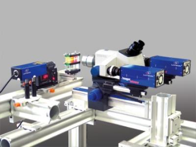
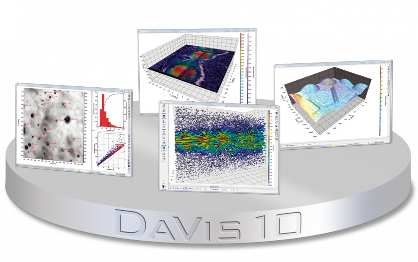
北京欧兰科技发展有限公司为您提供《预混漩涡火焰中显微层析PIV和甲醛的平面激光诱导荧光检测方案(CCD相机)》,该方案主要用于煤炭中显微层析PIV和甲醛的平面激光诱导荧光检测,参考标准《暂无》,《预混漩涡火焰中显微层析PIV和甲醛的平面激光诱导荧光检测方案(CCD相机)》用到的仪器有LaVision IRO 图像增强器、PLIF平面激光诱导荧光火焰燃烧检测系统、显微粒子成像测速系统(Micro PIV)、LaVision DaVis 智能成像软件平台。
我要纠错
推荐专场
CCD相机/影像CCD
更多


相关方案
-
方案 非预混火焰中5 kHz OH∗ 自发荧光和 OH 平面激光诱导荧光(OH PLIF)检测方案(CCD相机)
煤炭 | 5 kHz OH∗ 自发荧光和 OH 平面激光诱导荧光(OH PLIF)

- 查看全部方案
 咨询
咨询