

方案详情文
智能文字提取功能测试中
Robert R. Zarr, Victor Martinez-Fuentes,2 James J. Filliben, and Brian P. Dougherty' 294JOURNAL OF TESTING AND EVALUATION O 2001 by the American Society for Testing and Materials293 Calibration of Thin Heat Flux Sensors forBuilding Applications Using ASTM C 1130 By Robert R. Zarr and Brian P. DoughertyBuilding and Fire Research Laboratory Dr. James J. FillibenStatistical Engineering DivisionNational Institute of Standards and TechnologyGaithersburg, MD 20899-8632 USA And Victor Martinez Fuentes Division de Termometria Centro Nacional De Metrologia km 4,5 carretera a los Cues El Marques, Qro. 76241 Mexico Reprinted from the Journal of Testing and Evaluation, May2001. NOTE: This paper is a contribution of the NationalInstitute of Standards and Technology and is not subject tocopyright. Calibration of Thin Heat Flux Sensors for BuildingApplications Using ASTM C 1130 Authorized Reprint from Journal of Testing and Evaluation, May 2001 CCopyright 2001 American Society for Testing and Materials, 100 Barr Harbor Drive, West Conshohocken, PA 19428-2959 REFERENCE: Zarr,R. R., Martinez-Fuentes, V., Filliben, J.J.,and Dougherty, B. P.,“Calibration of Thin Heat Flux Sensors forBuilding Applications Using ASTM C 1130,” Journal of Testingand Evaluation, JTEVA. Vol. 29, No. 3, May 2001, pp. 293-300. ABSTRACT: Calibration measurements of thin heat flux sensorsfor building applications are presented. The findings support thecontinued development of precision and bias statements for ASTMPractice C 1130. Measurements have been conducted using a 1016mm diameter guarded hot plate apparatus (Test Method C 177) from10℃ to 50℃ and for a heat flux range of ±13 W/m.The option ofusing a 610 mm heat flow meter apparatus (Test Method C 518) tocalibrate the heat flux sensors is also explored. Experimental de-signs are presented to compare test methods, evaluate whichparameters affect the sensor output, and determine the functional re-lationship between the sensor output and applied heat flux. Thestudy investigates two sizes of sensors fabricated by one manufac-..turer. Sensor equivalency, grouped by size, is evaluated to deter-mine whether a calibration based on a subset of sensors will sufficeor if extensive individual calibrations are needed. KEYWORDS: building technology, calibration, guarded hotplate, heat flow meter, heat flux sensor, repeatability, thermal con-ductance, thermal insulation The National Institute of Standards and Technology (NIST) re-cently completed a series of calibration tests oftwelve thin heatflux sensors. The sensors are being used to investigate the thermalperformance of building-integrated solar photovoltaic panels [].The calibration data provide valuable information for the develop-ment of precision and bias statements for ASTM Practice forCalibrating Thin Heat Flux Transducers (C 1130). Practice C 1130describes experimental procedures for the calibration of heat fluxsensors for use on industrial equipment or building envelope com-ponents. For an application on an insulated building component,calibration at low levels of heat flux, on the order of 20 W/morless, is appropriate. This paper describes the heat flux sensors, test methods, and ananalysis of four calibration issues of interest to the user of C 1130:(1) sensor equivalency, (2) linearity and temperature effects,(3)uncertainty analysis, and (4) test method suitability. The issue ofsensor equivalency seeks to answer the question: can a calibrationdeveloped from a subset of sensors be used or are individual cali-brations required for each sensor? Another major objective of theanalysis is the investigation of the sensitivity and linearity of the ( Manusc r i p t r e ceived 6/16/ 2 000; ac c epted for pub lic ation 11/ 29 /2000. ) ( ' Mechanical engineer, N ational I n stitute of Standards and T e c hnology, 1 00 Bureau Drive, Gaithersburg . MD 2 0899-8632. ) ( M echan i cal engineer gu e st wo r ker , Nat i o n al C e nter of Metrology, Km 4 .5 C arretera a los C ues, E l M arques, Quere t a r o 76900, M e xico. ) ( M a t hematical stati s t i cian. Na t ional Institute of Standards an d Technol o gy,100 Bu reau D r i ve,Gaithersburg, M D 2 0 899-8980. ) sensors, and the effect of other factors, particularly temperature.An assessment of uncertainties for the calibration results is alsoprovided. The final section of the paper explores the option of us-ing two ASTM test methods for calibrating the same sensors. Background This section describes the heat flux sensors, ASTM test methods,and test protocols for calibration. Sensors Table 1 summarizes the physical characteristics of the heat fluxsensors. Each sensor utilizes a thermopile that produces an electrical voltage as a function of the heat flux through the metre area ofthe sensor. The underlying principle of operation is based on theSeebeck effect [2]. The sensors were manufactured using printedcircuit techniques so that the metal junctions of the thermoelementswere placed in the same geometric plane. In operation, thedifferent thermal conductivities of the constitutive elements perturb the local heat flux through the sensor’s metre area producing atangential temperature gradient [3] and electrical output voltage forthe sensor. ASTM Test Methods Practice C 1130 provides experimental procedures for the cali-bration of heat flux sensors. For this study, two test methods wereutilized-Test Method for Steady-State Heat Flux Measurementsand Thermal Transmission Properties by Means of the Guarded-Hot-Plate Apparatus (C 177) and Test Method for Steady-StateHeat Flux Measurements and Thermal Transmission Properties byMeans of the Heat Flow Meter Apparatus (C 518). Test method C177 is considered a primary (or absolute) method, whereas C 518is a comparative method since specimens of known thermal trans-mission properties are required for calibration of the apparatus. Thecalibration procedures for the C 518 apparatus are discussed in theliterature [4,5]. Table 2 summarizes the important characteristicsof each apparatus. Test Protocol The heat flux sensitivity, H (uV per W/m), is the ratio of thesensor’s output voltage, E (V), and the one-dimensional heat flux,q(W/m²), through its metre area, or When calibrating a sensor, q is provided by the test apparatus and,under steady-state conditions, is a function of the thermal conduc- TABLE 1—Heat flux sensors. Characteristics Small (A) Large (B) Quantity 9 3 Dimensions, mm 500 by 500 610 by 610 Metre area, mm 250 by 250 305 by 305 Nominal thickness, mm 0.8 0.8 Number of junctions 2500 3600 Nominal resistance,Q 1500 2250 Metal junctions Copper-Constantan Copper-Constantan Substrate material Glass-fiber reinforced epoxy Glass-fiber reinforced epoxy TABLE 2-Apparatus characteristics. C 177 C 518 Characteristics (Guarded Hot Plate) (Heat Flow Meter) Plate size, mm 1016 (diameter) 610 by 610 Metre area, mm 406 (diameter) 250 by 250 Time to achieve 8 4 steady-state,h Thtoot FIG. 1-Heat flux sensor tesi assembly. tance (C) of the specimen and the applied temperature difference(AT), The calibration temperature(T) is the average of the apparatus hotand cold surfaces. For C 177, q was obtained from the ratio of thespecimen heat flow (Q) and the metre area (A). The specimen heatflow (Q) was determined from the product of the metre area inputvoltage (V) and corresponding current (i). For C 518, q was deter-mined from the product of the apparatus calibration factor [4,5] andthe output voltage of the apparatus heat flux transducer. Each sensor was calibrated individually between adjacent layersof 3 mm silicone rubber (470kg/m) and 25 mm fibrous-glass ther-mal insulation (135 kg/m’) as shown in Fig. 1. This techniqueembedded the sensor in an assembly that provided a thermal con-ductance similar to the end-use application. The assembly was in-serted between the hot and cold plates of the apparatus, compresseda minimum of 2%, and tested with a steady temperature differenceapplied at the outer surfaces of the assembly. At the conclusion ofa test, the assembly was dissembled and the sensor removed. Thesame assembly materials were reassembled with a different sensorand the process repeated. Usually, the sensor’s metre area is calibrated within the perime-ter of the metre area of the apparatus. As noted in Tables 1 and 2,the metre areas of the small sensors are within or equal to the me-tre areas of the apparatus. For the large sensors, less than 1% of the sensor metre area is outside the metre area of C 177. Given thatmore than 99% of the sensor’s metre area is within the metre areaof C 177, the latter procedural deviation was considered small andsubsequently neglected. Unfortunately, approximately 33% of themetre area of the large sensors is outside of metre area of C 518 andthis deviation is discussed in the analysis. A thin thermocouple (copper-constantan) was installed at thecenter of each heat flux sensor to monitor the sensor temperature(T). The output voltages (E) and temperatures (T)) ofthe sensors,as well as q, T, and AT from the respective apparatus, were col-lected at 1 min intervals for 1 h using separate commercial dataacquisition systems. The standard uncertainties for the above mea-surements are discussed in the Appendix. As a side note, for building applications, the parameter of inter-est when utilizing heat flux sensors is the multiplicative inverse ofthe heat flux sensitivity, that is (1/H). The uncertainty contributionsassociated with end-use application are not addressed in this paper.However, for reference, other researchers have estimated the un-certainty for field applications to be as much as ±10% [6]. Analysis The analysis of data addressed four questions. First, can the sen-sors be treated equivalently in order to develop a global calibration(i.e., based on a subset of sensors), or are individual calibrationsrequired? Second, what is the functional form of the calibrationequation? Third, what is the standard uncertainty for the estimatesof H? Fourth, do Test Methods C 518 and C 177 yield equivalentresults for calibration? Sensor Equivalence: Global versus Individual Calibration The primary objective of the individual calibrations at fixed ther-mal conditions was to assess and quantify the equivalency of theheat flux sensors. If the sensors were, in fact, deemed equivalent, aglobal calibration could then be investigated. If not, a more exten-sive calibration would be required. A secondary objective was todetermine the repeatability of Test Method C 177 as part of Prac-tice C 1130. To determine repeatability, the same operators conducted replicate measurements for several sensors on differentdays.Completion of all measurements required nearly 30 days. To assess the sensor-to-sensor variation, individual measure-ments were conducted using C 177 at 20°℃ and a heat flux of 5.9W/m² through the assembly. For the test setup, the thickness of theassembly was preset to 58.9 mm, compressing the assembly by 2%.During the test, secondary factors such as the clamping force andchamber ambient humidity were monitored, but not fixed. Themean clamping force for all tests was 414 N ± 40 N (one standarddeviation) and the relative humidity was less than 10%. Table 3 gives the test data and summary statistics arranged bysensor size (A, B) for T, AT, q,Ti, E, and H. For consistency, anegative sign(-) has been assigned to values of q and AT whenvalues of E were negative. The summary statistics indicate thattest-to-test variations for the plate temperatures and correspondingheat fluxes (T, AT, and q) were quite small and that the coefficientsof variation (%CV) for H were also small,less than 1.3% for A and0.5% for B. The mean heat flux sensitivities (H) were 93.6uV/(W/m²) and 135.6 uV/(W/m²) for A and B sizes, respectively.The value of H for the small sensors is within 2% of results previ-ously reported by another researcher for a similar sensor [3]. Figure 2 plots the relative difference between values of E (Table3) and the group means (E) by sensor size (A, B). No apparenttrends are observed in the data. The maximum variation among the TABLE 3-Sensor-to-sensor variation using Test Method C 177. Date Heat Flux Sensor T,℃ AT,K q, W/m T℃ E. V H,pV/(W/m²) Sensor 11/03/99 A1 20.00 -10.00 -5.892 19.95 -0.000552 93.8 10/27/99 A2 20.00 -10.00 -5.873 19.96 -0.000562 95.7 11/15/99 A2 20.00 -10.00 -5.877 19.98 -0.000555 94.5 11/09/99 A3 20.00 -10.00 -5.911 19.94 -0.000552 93.4 11/16/99 A3 20.00 -10.00 -5.878 19.95 -0.000555 94.4 11/18/99 A3 20.00 -10.00 -5.879 19.95 -0.000555 94.4 11/22/99 A3 20.00 -10.00 -5.882 19.95 -0.000555 94.3 10/30/99 A4 20.00 -10.00 -5.891 19.95 -0.000542 92.1 11/17/99 A4 20.00 -10.00 -5.882 19.95 -0.000544 92.4 11/02/99 A5 20.00 -10.00 -5.905 19.97 -0.000540 91.5 11/01/99 A6 20.00 -10.00 -5.900 19.95 -0.000538 91.3 11/24/99 A6 20.00 -10.00 -5.874 19.95 -0.000540 91.9 10/31/99 A7 20.00 -10.00 -5.902 20.01 -0.000563 95.4 10/28/99 A8 20.00 -10.00 -5.872 19.99 -0.000546 93.0 10/29/99 A9 20.00 -9.99 -5.878 19.95 -0.000556 94.5 11/19/99 A9 20.00 -10.01 -5.888 19.95 -0.000553 93.9 11/05/99 B10 20.00 -10.00 -5.883 19.95 -0.000798 135.7 11/08/99 B1] 20.00 -10.00 -5.900 19.94 -0.000796 134.9 11/23/99 B11 20.00 -10.00 -5.884 19.94 -0.000797 135.5 11/04/99 B12 20.00 -10.01 -5.907 19.94 -0.000806 136.4 Summary Statistics (A,B) Mean A 20.00 -10.00 -5.886 19.96 -0.000551 93.6 Std. A 0.002 0.004 0.012 0.018 0.000007 1.2 % CV A 0.0 -0.1 -0.2 0.1 -1.2 1.3 Mean B 20.00 -10.00 -5.894 19.94 -0.000799 135.6 Std. B 0.002 0.003 0.012 0.002 0.000005 0.6 % CV B 0.0 -0.0 -0.2 0.0 -0.6 0.5 Heat Flux Sensor FIG. 2-Sensor-to-sensor variation using Test Method C 177:(AT=-10K,T=20℃,q=-5.9 W/m’). small sensors (A) was less than ±2.5% and for the large sensors(B) less than ±1%. Given that the relative differences in Fig. 2 andcoefficients of variation for H (Table3) are small in comparison tothe uncertainties of the end-use application(±10%)[6], we con-clude that the sensors are equivalent and thus a global calibrationamong sensor sizes is appropriate. By pooling replicate data and weighting with their respective de-grees of freedom, the repeatability standard deviations were deter-mined to be 0.53 pV/(W/m²) (0.6%) and 0.40 pV/(W/m²) (0.3%) for A and B sensors, respectively. The larger value is used later todetermine the combined standard uncertainty for H. Calibration Curve The purpose of this section is to develop a calibration curve thatrelates E and q. i.e., E =f(q). In this regard, the following ques-tions are addressed:(1) Are other variables needed, in particular Tto fully relate E and q, i.e., E =f(q,T)? (2) Is an interaction term qT needed? (3) If q itself is sufficient, is the relationship between Eand q linear? and, (4) If linear in q, is an intercept term needed? Temperature Effect on the Calibration-Other researchers [7]have identified various parameters that can affect the sensor output(E). These parameters include heat flux (q), temperature (T),clamping force, thermal conductivity of surrounding material(s),surface air velocity, emittance of the sensor and surrounding mate-rial(s), moisture, and installation.Other parameters not specificallymentioned could also affect sensor output but are not considered inthis study. The objective of this part of the study was to determinethe effect of two such factors, q and T. Note that q was varied byindirectly controlling a surrogate parameter, that is, the AT acrossthe assembly. A complication was that the thermal conductance(C) of the assembly is a function of temperature (i.e., C=C(T)),and therefore changes in T also affected q and therefore E (see Eqs1 and 2). The findings from the previous section permitted the selection ofa subset of sensors for full characterization as a function of q andT. Therefore,two small sensors were selected randomly and testedindividually in the same assembly (Fig.1) using C 177 at four lev-els each of q (AT) and T. The ranges for q (±13 W/m) and T(10to 50°C) were selected to represent end-use conditions. For the testsetup, the thickness of the assembly was again preset to 58.9 mm,compressing the assembly 2%. The clamping force and thicknessvaried with temperature due to thermal expansion effects from testto test. Table 4 summarizes the test results for the 16 tests. For consis-tency, a negative sign (-) has again been assigned to values of q(and A7) for negative values of E, indicating a change in the direc-tion of heat flow. The choice for electrical polarity was entirelyarbitrary; inverting the sensor changes the direction of heat flowand produces a positive signal. The data in Table 4 were fit to the following model where q is the heat flux (W/m), T is the sensor temperature (C),a; are the regression coefficients, and e is a random error term. Totest the statistical significance of the estimates for the individual re-gression coefficients, 95% confidence intervals (CI) were con-structed for aj. The form of the confidence interval is TABLE 4-Effect oftemperature and heat flux on small sensors (A). Heat Index Flux Sensor T.C ATK q. W/m T,℃ E. V 10.00 -20.00 -11.443 10.20 -0.001079 50.00 -20.00 -13.266 49.76 -0.001245 10.00 19.99 11.464 10.29 0.001080 50.00 -20.00 -13.253 49.71 -0.001240 10.00 20.00 11.465 10.21 0.001073 50.00 20.00 13.14] 49.89 0.001240 10.00 -20.00 -11.465 10.18 -0.001080 50.00 20.00 13.161 49.87 0.001244 20.00 -10.00 -5.881 20.01 -0.000560 39.99 -10.01 -6.344 39.79 -0.000595 20.00 10.00 5.874 20.00 0.000554 40.00 9.99 6.309 39.90 0.000597 20.00 -10.00 -5.871 19.97 -0.000558 40.00 -10.00 -6.332 39.82 -0.000601 20.00 10.00 5.865 20.05 0.000561 40.00 10.00 6.330 39.83 0.000594 TABLE 5-Hypothesis test for statistical significance ofregressioncoefficients. -3.91E-06 9.43E-05 1.44E-07 -3.03E-09 Std(a) 2.55E-06 2.48E-07 7.54E-08 6.68E-09 10.975、11-P 2.145 2.145 2.145 2.145 95%C1- -9.38E-06 9.38E-05 -1.71E-08 -1.74E-08 95% C1+ +1.56E-06 9.48E-05 +3.06E-07 +1.13E-08 Conclusion Insignificant Significant Insignificant Insignificant where n (= 16) is the number of data points, p (=4) is the numberof parameters in Eq 3,to.975.n-p is the 97.5 percentile of the Stu-dent’s t-distribution with n - p degrees of freedom, and Std(a;) isthe standard deviation of the estimated regression coefficient a;. Ifthe interval defined by Eq 4 contains zero, then the coefficient ofinterest is statistically insignificant at the α=0.05, where 95% =100(1-a). From Table 5, at a=0.05, we conclude that only theq coefficient (a:) is statistically significant. Unfortunately, the confidence interval technique alone cannotdetect the presence of a temperature effect if subtle. For this case,further analysis is required. Using the results from Table 5, we ten-tatively assume the simple model, E = aq, and fit this model withthe data from Table 4. If this model is entirely adequate, the devia-tions (defined as the differences of the data and predicted values)should be random, without structure, when plotted against the othervariables, such as T or qT. Conversely, if the model is inadequate,the deviations will exhibit a deterministic structure when plottedagainst such contributing variables. Figure 3 plots the deviations (from the E=a;q fit) versus T andqT, respectively. A subtle temperature dependence is evident inFig. 3a. In particular, the four deviations at 10°C are smallerthan the four deviations at 50°C. No similar effect is noted for qT(Fig.3b). There are apparently two contradictory conclusions for the tem-perature effect on calibration. The effect is insignificant by the con-fidence interval test, yet significant for the simple model residualanalysis. Our final conclusion was determined by comparing theresidual standard deviations (SREs) for the two models shown inTable 6. The residual standard deviation is a measure of qualityof fit. From Table 6. we see that the absolute difference of includingthe temperature effect improved the fitted model by only a smallamount, 0.4 pV. Therefore, the term T (and qT) was omitted insubsequent analyses. It should be noted that the conclusion regard-ing the statistical insignificance of T applies only to the relativelynarrow temperature range under study and such conclusions maynot necessarily apply to larger temperature ranges or other types ofsensors. Form of Calibration Equation-A major objective of this studywas to assess the linearity of the sensor output (E) with respect toq. Additional calibration measurements were conducted for thelarge (B) sensors. Based on the analysis of the temperature effect,the large sensors were tested at 20°C and four different levels ofheat flux. Table 7 summarizes the results for the six tests. The data from Tables 3, 4, and 7 are combined and values of Eplotted as a function of q(Fig.4a). The plot indicates that E was,in fact, a linear function of q for both small (A) and large (B) sen-sors. The data for A and B sensors were fit to an equation of theformE=E,+ Hq shown as solid lines in Fig. 3a. The interceptterm was included to check the significance of our previous results. FIG.3-Deviations versus independent parameters, T and qT, for model E=Hq. TABLE 6—Comparison of models. Model SRES.uV E=01q 5.0 E=ao+ajq+aT+ayqT 4.6 TABLE7-Additional data for large sensors. lndex Heat Flux Sensor T.℃ AT.K q.W/m E.V B12 20.00 10.00 5.867 19.99 0.000810 2 BII 20.00 -20.00 -11.837 20.01 -0.001616 3 B10 20.00 10.00 5.855 n.r.* 0.000802 4 Bl1 20.00 -10.00 -5.872 19.94 -0.000801 5 B11 20.00 10.01 5.871 19.97 0.000799 6 BII 20.00 20.00 11.829 20.09 0.001617 Figure 4b shows the deviations (%) from the curve fit (E) versusg. The deviations for all twelve sensors are less than ±3%, and ran-domly scattered about zero indicating a satisfactory fit. The neces-sity for an intercept term can be investigated further by using acurve fit of the form E =Hq. Results for the small and large sen-8b. The estimates for H, corresponding standard deviations (Std(H)),and residual standard deviations for the fit (SREs) given in Tables8a and 8b confirm that the intercept term is not required and thefunctional form ofE = Hq is sufficient. Global versus Individual Calibration (Revisited)-Another ma-jor objective of this analysis was to confirm our previous results forsensorequivalency by examining the curve fits for different groupsof sensors. Tables 9a and 9b summarize the curve fit statistics forsmall and large sensors (A and B), respectively. TABLE 8a-Statistical fit parameters for functional form:E=Eo + Hq. Parameter (Units) Small Sensors Large Sensors A1-A9 B10-B12 32 10 Eo(pV) 1.9 3.4 Std(Eo)(pV) 1.29 1.40 H(pV/(W/m)) 94.1 136.5 Std(H) (uV/(W/m)) 0.16 0.19 SRES (pV) 6.8 4.4 TABLE 8b-—Statistical fit parameters for functional form: E= Hq. Small Sensors Large Sensors Parameter (Units) A1-A9 B10-B12 72 32 10 H(uV/(W/m²)) 94.0 136.4 Std(H) (pV/(W/m²)) 0.15 0.23 SRES (pV) 6.9 5.4 TABLE 9a-Statistical fit parameters for small sensors (A): E=Hq. Parameter A2 A7 A2&A7 A1-A9 12 H (p.V/(W/m²)) 10 9 19. 32 94.1 94.4 94.3 94.0 Std(H) (pV/(W/m²)) 0.17 0.18 0.13 0.15 SRes(uV) 5.0 5.0 5.2 6.9 TABLE 9b-Statistical fit parameters for large sensors (B):E= Hq. Parameter (Units) B11 B10&B1I B10-B12 11 6 8 10 H(pV/(W/m²)) 136.3 136.3 136.4 Std(H)(uV/(W/m²)) 0.25 0.22 0.23 SRES (pV) 5.1 4.7 5.4 The estimates for H, corresponding standard deviations (Std(H)),and residual standard deviations for the fit (SREs) given in Tables9a and 9b are quite similar. From an engineering perspective, theresults confirm that, across groupings by size, the small and largesensors (A,B) were equivalent. Final Calibration Equations-In summary, the final calibrationequations for the small (A) and large (B) sensors were (1) E=94.0q, and (2)E=136.4q, respectively. Uncertainty Analysis The uncertainty for the calibration results was evaluated usingcurrent international guidelines [8,9] for the expression of mea-surement uncertainty. The measurement uncertainty for the esti-mate of H can be determined by consideration of three primarycomponents: the standard uncertainties for the regression analysis,replication, and the individual measurement contributions. Thecomponents are combined by the method of propagation of errors,Or Here, u is the standard uncertainty of regression coefficient(Std(H)) given in Table 8b, u2 is the standard uncertainty for repli-cate measurements, and us is the standard uncertainty for the mea-surement estimate of H (see Appendix). The standard uncertainty for the regression coefficient is takenas the larger of the values given in Table 8b,0.23 pV/(W/m). Thestandard uncertainty for the replicate measurements is 0.53pV/(W/m) as given earlier. The standard uncertainty for the mea-surement estimate of H includes uncertainty contributions from Eand q and is determined to be 1.4 pV/(W/m²)as shown in the Ap-pendix. The combined standard uncertainty (Eq 5) is thus 1.5pV/(W/m²) or, in relative terms, 1.6 and 1.1% for the small andlarge sensors, respectively. Comparison of Test Methods The primary objective of the comparison was to assess and quan-tify the equivalency of the test methods. A secondary objective wasto quantify the effect of sensor size on H. Four sensors, two fromeach group in Table 1, were selected randomly and tested daily ina random sequence using C 518 at 24C and 13 W/m. Only onesensor from each group was tested using C 177. The sensors weretested in each apparatus with the same direction of the heat fluxthrough the sensor. Table 10 summarizes the results. The differences between theaverage values of H obtained from C 177 and C 518 were -1.1%for A4 and -2.0% for B12. The maximum within-method rangesfor H were 0.7% and 1.8% for C 177 and C 518, respectively. Bycomparison,the “best"expected imprecision indices for C 177 andC 518 are 2 and 3% (2 standard deviation level),respectively.Therefore, the differences between test methods could be consid-ered statistically “equivalent" for many applications. The calibra-tions presented herein, however, were conducted using C 177because of the size limitations of C 518 and the requirement for ad- TABLE 10—Calibration test method comparison (24℃,AT =22 K). C 177 C 518 Sensor )7 H (p.V/(W/m²)) Range (%) H (pV/(W/m²)) Range (%) Difference (%) 2 91.4 0.7 92.4 -1.1 94.3 B10 138.3 B12 136.8 0.4 139.5 -2.0 ditional calibrations of the apparatus as a function of temperature.As noted in Table 10, values of H for the large sensors (B) are about49% greater than the small sensors (A). Conclusions This paper addresses four primary issues of interest to the user ofC 1130 for the calibration of heat flux sensors for building applica-tions. The calibration measurements were conducted using TestMethod C 177 from 10 to 50C and for a heat flux range of ±13W/m’. The twelve sensors were found to be sufficiently equivalentamong size categories to allow calibration using a subset ofsensors, thus avoiding an extensive calibration requiring many in-dividual measurements. The calibration curve is a linear functionthat directly relates the sensor output to the applied heat flux. Thefunction does not require an intercept term. The final calibrationequations for the small and large sensors are E = 94.0q and E=136.4q, respectively. The relative combined standard uncertaintiesare estimated to be 1.6 and 1.1% for the small and large sensors,respectively. Additional information was determined for the development ofprecision and bias statements for Practice C 1130. Using TestMethod C 177, the repeatability standard deviations determined bypooling data for replicate measurements among small and largesensors were 0.53 pV/(W/m²)(0.6%) and 0.40p.V/(W/m)(0.3%),respectively, at 20℃ and 5.9 W/m’. A comparison of Test Meth-ods C 177 and C 518 indicated agreement within 2%, or better,at24℃ and 5.9 W/m². Furthermore, the calibration results obtainedusing C 177 for the small sensors were within 2% of previous re-sults [3]. In view of these results, this particular type of heat fluxsensor may serve as a candidate for future interlaboratory testing todetermine reproducibility precision indices for Practice C 1130. Acknowledgments The authors appreciate the assistance of Susan M. Fioravantewith the measurements. APPENDIX The combined standard uncertainty for the measurement esti-mate of H was determined by application of the law of propagationof uncertainty to Eq 1: The sensitivity coefficients, ci, are the partial derivatives of Eq lwith respect to E and qevaluated at their respective input estimates.Recall that for C 177, qwas determined directly from the electricalpower input (Q) to the apparatus metre area divided by metre area(A), or q=Q/A. The combined standard uncertainty for the mea-surement estimate of q was determined from The uncertainty budget for the determination of qis given inTable A1. The estimates for Q and A were 0.7636 W and 0.129748m’. The standard uncertainty for u() was taken from a previousseries of experiments [10]. The uncertainty budget for the determination of H is given inTable A2. The estimates used for E and q were 0.000551 V and5.866 W/m². The combined standard uncertainty for the measuresment estimate of H was 0.0000014 V/(W/m²), or 1.4 pV/(W/m). TABLE A1—Summary of standard uncertainty components for q. Source of Uncertainty C (1) repeated observatjons 0.00050 W 1 (pooled), u(Qmean) (2) uncertainty of voltage, current 0.00083 W 1 measurements,u(V, i) (3) deviation from one-dimensional heat flow,u(Q) (4) combined standard uncertainty,u(Q) (5) metre area, u(A) Combined standard uncertainty, u(q) 0.00980 W 1 0.00985 W 1/A 0.000023 m² 0.0759 W/m -Q/A TABLE A2-Summary of standard uncertainty components for H. Source of Uncertainty C: (1) repeated observations (pooled), 0.000002 V u(Emean) (2) digital voltmeter, u(E ) -0.000002 V (3) offset voltage for connection 0.000003 V card,u(E2) (4) combined standard uncertainty, 0.000004V 1/g u(E) (5) combined uncertainty,u(q) 0.0759 W/m -E/q Combined standard uncertainty, u(H) 0.0000014 V/(W/m²) ( R e f e r ence s ) ( [/ ] F an n ey, A . H . a nd Dou gh erty, B . P., “ B uilding I n t egr a ted P hot o voltaic Test F a c ility,"Proceedings of th e ASES, N P SC,AIA, ASME, M REA Co n ference So l ar 2000, 16-21 Ju n e 20 0 0. ) [2] Manual on the Use of Thermocouples in Temperature Mea-surement; ASTM Manual 12, ASTM, Philadelphia, PA, 1993. [3] Degenne, M. and Klarsfeld, S.,“A New Type of HeatFlowmeter for Application and Study of Insulation and Sys-tems," Building Applications of Heat Flux Transducers,ASTM STP 885, E. Bales, M. Bomberg,and G. E. Courville,Eds., American Society for Testing and Materials, Philadel-phia, 1985, pp. 163-171. [4] Zarr R. R., “Control Stability of a Heat-Flow-Meter Appara-tus," Journal of Thermal Insulation and Building Envelopes,Vol.18, October 1994, pp. 116-127. [5] Lackey, J., Normandin, N., Marchand, R., and Kumaran, K.,“Calibration of a Heat Flow Meter Apparatus,” Journal ofThermal Insulation and Building Envelopes, Vol. 18, October1994, pp. 128-144. [6] Flanders, S. N., “Heat Flow Sensors on Walls-What CanWe Learn?"Building Applications of Heat Flux Transducers,ASTM STP 885, E. Bales, M. Bomberg,and G. E. Courville,Eds., American Society for Testing and Materials, Philadel-phia, 1985, pp. 140-159. [7] Powell, F. J. and Rennex, B. G., “Workshop on LaboratoryUse of Heat Flux Transducers,” Building Applications ofHeat Flux Transducers, ASTM STP 885, E. Bales. M.Bomberg,and G. E. Courville, Eds., American Society forTesting and Materials, Philadelphia,1985,pp.245-249. [8] ANSI,“U.S. Guide to the Expression of Uncertainty in Mea-surement,”ANSI/NCSL Z540-2-1997, 1997. [9] Taylor, B. N. and Kuyatt, C. E., “Guidelines for Evaluatingand Expressing the Uncertainty of NIST Measurement Re-sults,”NIST Technical Note 1297. 1994. [10] Zarr,R. R., “Glass Fiberboard, SRM 1450c, for Thermal Re-sistance from 280 K to 340 K," NIST Special Publication260-130,1997.
关闭-
1/9

-
2/9

还剩7页未读,是否继续阅读?
继续免费阅读全文产品配置单
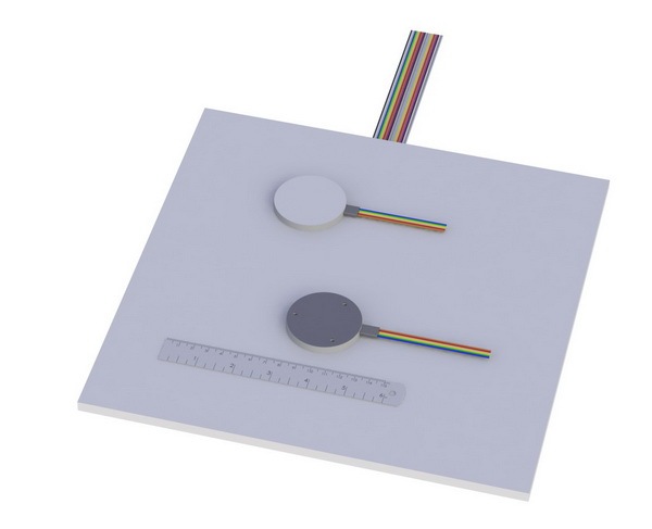
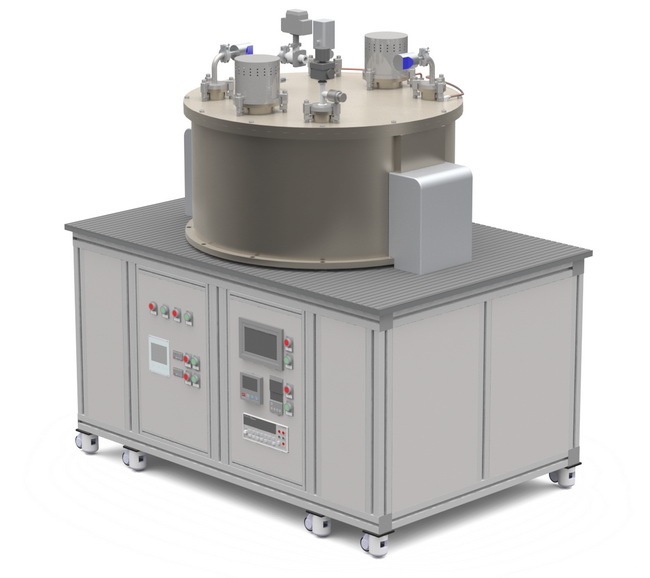
上海依阳实业有限公司为您提供《依据ASTM C1130校准建筑行业中使用的薄型热流传感器》,该方案主要用于建筑工程中检测,参考标准《暂无》,《依据ASTM C1130校准建筑行业中使用的薄型热流传感器》用到的仪器有高灵敏度热阻式热流计、高温热流计法导热系数测试系统。
我要纠错
推荐专场
相关方案
 咨询
咨询