方案详情文
智能文字提取功能测试中
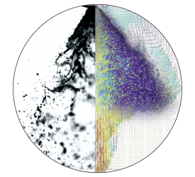
-114 CA Analysis of Hydrogen Direct-Injection Internal Combustion Engineswith Methods of Computational Fluid Dynamics U. Gerke, K. Boulouchos, A. Wimmer, W. Kirchweger Abstract Hydrogen direct-injection (DI) engines offer a wide range of possibilities forcombustion design, such as fuel stratification and multiple injections. Combustionmay involve premixed, partially premixed and non-premixed modes. Key issue of anon-homogeneous engine operation is an accurate preparation of the fuel/airmixture. Optical investigations and three-dimensional numerical analysis are appliedwith regard to an improvement of the injection parameters and combustion process.The present work outlines results of Computational Fluid Dynamics (CFD) withrespect to mixture formation and combustion in comparison to experimental data.Special emphasis is given to the influence of turbulence models on mixture formationcalculations. As to CFD simulation of stratified operation, the hydrogen mixture formation is ofcrucial importance for the subsequent fuel conversion. Consequently, numericalanalysis of the combustion process can only be as accurate as the computation ofthe mixture distribution it is based upon. Main influence on mixture formationcalculations of hydrogen-jet propagation was recognised to be the numerical grid aswell as the turbulence modelling approach. The influence of molecular diffusion onthe hydrogen mixture formation process was found to be negligible. The performedCFD analysis discusses different two-equation turbulence models as well as aReynolds Stress Model approach. The influence of the models on results of mixtureformation and turbulent kinetic energy (velocity fluctuations) is demonstrated. CFDresults are validated against optical experimental data from a research engine, usingplanar laser induced fluorescence (PLIF) measurements. Results of combustion analysis are depicted in terms of pressure traces and burnrates. CFD-results of both port fuel injection and direct injection operation arecompared to experimental data for stoichiometric mixtures at 2000 rpm. A turbulentflame speed closure approach is applied as combustion model, where the meanreaction progress is depicted in terms of a transport equation of a progressvariable . Regarding description of the turbulent flame speed, a model based onlaminar flame speed data as proposed by Zimont (1999) is applied. 1. Introduction The rapid progress in fuel direct-injection technology within the last decade alsoproved to be advantageous for hydrogen internal combustion engines. Equivalent totoday’s conventionally fuelled engines, state-of-the-art direct-injection technologyalso allows hydrogen engines to arrange specific combustion characteristics, e.g. fuelstratification and multiple injections of dedicated amounts of fuel. Depending on theinjection strategy, the mixture formation of hydrogen high-pressure (~150 bar) direct-injection engines (DI) is not limited to premixed combustion present in port fuelinjection engines (PFI), but allows a combination of premixed, partially premixed andnon-premixed diffusion-controlled flames. Phenomena such as pre-ignition, knocking and the air-displacement effect, generally known as disadvantages of PFI hydrogenengines, may be avoided by the use of hydrogen direct injection. Additionally,specific power and fuel efficiency may be increased and nitrogen oxide rawemissions may be lowered by the employment of this technology. A summary of thecapabilities of state-of-the art hydrogen DI engines is given in the report of Gerbig etal. (2004). Additionally, results regarding supercharged operation may be found inthe recent report of Grabner et al. (2006). The complexity of hydrogen DI operation requires a fundamental knowledge aboutthe in-cylinder processes in order to improve the combustion concept. Consequently,a deepened understanding of mixture allocation and flame propagation may beacquired by the application of advanced development methods such as opticalexperimental methods, e.g. Planar Laser-Induced Fluorescence (PLIF), andnumerical analysis in terms of three-dimensional Computational Fluid Dynamics(CFD). While CFD methods are still being researched, the results achieved from theemployed optical methods may directly be used to improve engine design.Accordingly, in the present work PLIF is consulted to validate results obtained bynumerical analysis, e.g. to verify the influence of different turbulence models onmixture formation calculations. To ameliorate the understanding of the employed PLIF technique, a description ofthe optical research engine is given in the following. Section 3 explains feasibleoperating strategies for the hydrogen direct-injection combustion concept. Thecomputational model is presented in section 4 including a description of theemployed numerical grid and theory on the applied turbulence models. In section 5CFD-results of mixture formation analysis are presented, whereas grid influence istaken into consideration and numerical results of different turbulence models arecompared to PLIF measurements. Additionally, velocity fluctuations predicted by theinvestigated turbulence models will be discussed comparatively. Computationalresults of combustion analysis are shown in section 6. Concluding remarks are listedin section 7 of this paper. 2.. Description of research engine Subject of investigation is a four-valve, 0.5 litre spark-ignited single-cylinder researchengine with adjustable compression ratio. Geometrical dimensions are 84 mm boreand 90 mm stroke. Measurements of indicated tracnaust gii aniYiliiries and exhaust gas analysis areconducted on a thermodynamic research engine with a maximum engine speed of7000 rpm. In the present work a magnetically actuated high-pressure gas injectorwith lateral orientation is emploved for hydroqen injection. The injector nozzlegeometry features eight holes with a diameter of d=0.4 mm each resulting in ageometric flow area of A=1 mm. The supply pressure of hydrogen is p= 150 barwhich allows shortened injection duration due to the increased density of the highpressure gas and thus permits wide limits of injection timing, e.g. injecting into thecompressed charge during compression stroke. The maximum steady hydrogenmass flow is 6.5E-03 kg s. The spark plug is located in the centre of the combustionchamber. PLIF-measurements are carried out on a particular version of the research enginethat allows optical access into the combustion chamber. The engine is thereforeequipped with a quartz glass cylinder liner of 44 mm height located below thecylinder head, and an additional quartz glass window embedded in the piston. Theglass cylinder is shaped in line with the contour of the cylinder head dome in order to Bore / Stroke 86 /86 mm Displacement 499.6 cm³ Compression ratio 9.1 Max. speed 2000 min' Max. cylinder pressure 60 bar Glass liner height 44 mm Fuel tracer Triethylamin (TEA),200 ppm LIF Laser System KrF-Excimer laser,248 nm Camera System LaVision Imager3s CCD,intensified relay optics Figure 1: Model of the optical research engine with laser beams passing through theglass ring and the piston window separately. The resulting laser sheet illuminates thevertical symmetry plane of the combustion chamber. achieve a maximum side visibility of the area around the spark plug and the injectornozzle. An optimized illumination of the combustion chamber is gained by splittingthe laser beam into two single beams passing through the glass ring and the piston-window separately. A vertical light sheet is produced which incorporates the cylinderaxis and is perpendicular to the crank axle. The illuminated plane includes the twopossible injector positions (lateral and central) and the location of the spark plug, cf.Figure 1. The engine speed of the optical research engine is limited to 2000 rpm, thecompression ratio is 9.1:11 and the maximum in-cylinder pressure is 60 bar.Consequently, the engine may be operated using practical operating points in firedmode. In order to assure compatibility of results, the optical research engine featuresapproximately the same geometric properties as the thermodynamic version. To visualise hydrogen distribution during mixture formation process a tracersubstance has to be admixed to the fuel. Hydrogen applications require particulartransport properties of the tracer so that demixing may be avoided. Followingconsiderations of Blotevogel et al. (2003) in the present investigation Triethylamine(TEA) was chosen as a suitable tracer substance. The tracer can be excited by laserlight at a wavelength of 248 nm using a Krypton-Fluoride (KrF) excimer laser. Thefluorescence signal of the tracer is recorded with a CCD-camera allowing aquantitative determination of hydrogen concentration. Regarding the visualisation ofthe combustion process either excitation of OH-radicals or tracer-measurements areemployed. Relating to the first method, the passing flame front is detected by OH-fluorescence. Relating to the latter method, the unburned zone is visualized bytracer-fluorescence while in the burned zone the tracer is consumed by the flame andthus is not visible anymore. For comparison with CFD-results in terms of ReynoldsApproximated Navier-Stokes (RANS), experiments are averaged over 50 cycles. Adetailed description of the applied PLIF measurement technique is published in thereport of Kirchweger et al. (2006). 3. Influence of injection timing on mixture formation Hydrogen internal combustion engines offer a wide range of possible operatingstrategies. Due to the extensive ignition limits of hydrogen, an unthrottled operation ina quality-controlled mode is feasible. Additionally, high pressure direct-injectionaffects fuel-mixture preparation, which may be influenced by injection timing.Accordingly, the start of injection (SOI) is the most representative parameter forhydrogen DI. Different combustion modes have to be distinguished, depending on start, durationand quantity of fuel injections. Regarding single injection events a premixedcombustion regime, comparable to PFl, is present when fuel injection is located atthe beginning of the compression stroke, e.g. SOI=-120 CA (with respect to topdead centre, TDC). In this case large timeframes for the fuel/air mixture preparationexist. A partially premixed combustion mode may be obtained when timeframes forthe fuel/air mixture preparation decrease, e.g. when the injection event is locatedclose to the end of the compression stroke (e.q. SOl=-20 ℃A). The mixingtimeframes and thus the degree of air/fuel stratification are directly related to SOl.The end of injection (EOl) is located prior to spark ignition and consequently thecombusisttiioonn proceeds iinn a propagation-flame manner comparably to gasolineengines. Regarding multiple injection events it has to be distinguished whether secondaryinjection takes place prior to or after ignition timing. The former type is referred to aspropagation-flame combustion modes described above for single injection. Here,several injections may be used to improve either mixture homogenisation orstratification. Latter types result in a diffusion-flame combustion mode which iscaused by fuel injection into the flame front of a previously generated spark ignitedpropagation flame. This mode, referred to as combustion control, is comparable to acombined gasoline/Diesel engine type process (non-premixed, diffusion flame mode)and may be realised with various numbers of discrete injection events. The differentportions of injected fuel may be expressed in terms of individual values of fuel/airequivalence ratio, e.g. oi and g2 belong to the first and second injection event,respectively. The global fuel/air equivalence ratio is then given by d= 01 + 02. 4. Computational model 4.1. Numerical grid The physical domain is discretised with an unstructured tetrahedral grid and prismaticlayers at the wall boundary. Due to the lateral, symmetric position of the hydrogeninjector a symmetrical flow fieldIsassumed.This assumption allowsthecomputational domain to be modelled as one half of the physical domain only. Thevertical plane through the injector’s central axis is defined as a symmetry plane, cf.Figure2 where the mesh topology of the cylinder and injector nozzle is shown. Thefire land of the piston is not modelled. The compression ratio of 9.1:1 is adjusted inthe CFD model. Considering the computation of the supersonic hydrogen jet and high velocitygradients at the hydrogen inflow the resolution of the numerical grid around theinjector nozzle is refined systematically. A compromise of a grid resolution that issufficient for a proper description of the flow field and also results in acceptable CPUdemands was achieved. This grid is identified as Standard Grid, dedicated to beused as a standard for hydrogen DI mixture formation computations. The size of tetrahedral elements in the outer flow field of this grid is 3 mm. The resolution in thearea of the injector’s holes is refined to an element size of 0.05 mm (16 elements perpipe). From the injector wall to the in-cylinder flow the size of tetrahedral elements isincrementally increased within four zones from 0.05 to 0.25,0.5 and 1 mm. Theboundary layer of the grid is modelled with 4 prismatic layers of 0.05 to 0.2 mmheight. Depending on the position of the piston, the overall number of cells of thecomputational domain counts approx. 3 million elements. Compared to computations with even more refined meshes, effects of numericaldiffusion may not be eliminated completely with the Standard Grid. Conclusions of aninvestigation of the influence of numerical grid resolution on computational results aredemonstrated in section 5.1 where CFD-results of mixture formation employingdifferent numerical grids are compared. Figure 2: Element distribution of the Standard Grid at the area of the injector’s inflow(cross section). The size of tetrahedral elements in the bore is 0.05 mm. From theinjector wall to the inner flow field the element size is incrementally increased withinfour zones from 0.05 to 0.25, 0.5 and 1 mm for the Standard Grid. 4.2. Initial and boundary conditions Information for initial and boundary conditions for the computational model is takenfrom experimental measurements; and one-dimensional engine cycleprocessanalysis. Results from CFD-simulations of the exhaust and intake stroke areconsidered as initial conditions for the computation of compression stroke andhydrogen injection. At the beginning of the exhaust stroke the cylinder is initialised with burned gasmixture. The intake and exhaust port boundary conditions of the CFD model aregiven by unsteady pressure and temperature conditions taken from engine cycleprocess analysis. Regarding hydrogen injection a mass flow inlet boundary conditionis defined. With the assumption of proportionality between needle lift and mass flow,the profile of the hydrogen mass flow boundary condition is derived from the start ofinjection (SOI) and the end of injection (EOl). The absolute value of the injected fuelmass is used to define a representative trapezoid profile which is finally used as aboundary condition for the CFD computation as a function of crank angle. 4.3. Turbulence modelling In order to verify the closure of Reynolds stresses different approaches for turbulencemodelling are employed. Firstly, two-equation models based on eddy viscosityhypothesis,e.g. Renormalisation Group (RNG) k-eand Shear Stress Transport (SST) turbulence models are compared. Secondly, a so-called Reynolds Stress Model(RSM) is investigated, which is a higher (second) order modelling approach. In the two-equation turbulence models for the closure of the turbulent kineticenergy k and the dissipation rate e two balance equations have to be solved. TheRNG k-8 approach derived by Yakhot& Orszag (1986) is based on RenormalisationGroup (RNG) analysis of the Navier-Stokes equations. In comparison to the standardk-e model, constants differ and one constant in the -equation is replaced by ananalytic function. Details regarding this approach may be found in the publication ofYakhot & Orszag. The SST (Shear Stress Transport) model developed by Menter (1993) combines thek-e and the k-ω approach by use of a blending function and thus should providehigher accuracy for boundary layer simulations than the standard k-e model. Themodel operates by solving a turbulence/frequency model (k-ω) at the wall and k-e inthe outer part of the flow, where k-a and k-a models are combined by a blendingfunction that ensures a smooth transition between the two approaches. For freeshear flows, the SST model is identical to the k-a model. A detailed description of theSST model is published in the report of Menter. Both two-equation models (RNG k-:and SST) are industrial standard and result in reasonable computational costs. The Reynolds stress turbulence model (RSM) is a more sophisticated approachcompared to two-equation models since the individual components of the Reynoldsstresses and the dissipation rate are solved. In contrast to the two-equation modelsbased on eddy viscosity hypothesis, the RSM does not assume isotropic turbulenceand thus anisotropic features of in-cylinder turbulent flow are better represented. Inparticular swirling flows as present with direct-injection of hydrogen are said to bewell represented by the herein investigated model derived by Speziale et al.(1991).This model uses a second-order description for the pressure-strain correlation of thetransport equations in the Reynolds stresses. However, numerical costs of the RSMapproach are increased due to the solution of additional transport equations whichlimit the everyday applicability of this approach. Additionally, numerical instabilitiesmay lead to convergence problems with this model. A detailed comparison of hydrogen DI mixture formation calculation regarding thedifferent turbulence models against optical measurements is given in section 5.2. 5. Mixture formation analysis Among all operating points of an in-cylinder hydrogen-mixture formation process, themost challenging one for CFD investigations is injection with SOl right after intakevalve closing (early injection). In this configuration nearly the complete time of thecompression stroke is available for the mixture process where the hydrogen jetpropagates as a swirl in a cylindrical path through the combustion chamber (walleffects and free shear flow). Depending on the amount of injected fuel a ratherhomogeneous air/fuel mixture distribution is obtained at the end of the compressionstroke. Concerning a stratified load, hydrogen injection with SOl close to top deadcentre (TDC) is investigated. In the following, for an estimation of error due to..:LLnumerical diffusion a grid comparison with refined computational meshesisemployed and a comparison of mixture formation calculations with differentturbulence models for injection timing of SOI=-120 CA with respect to TDC isgiven. In the present investigation PLIF measurements which provide excellentinformation about the mixture distribution with high resolution in space and time areused for validation of CFD simulation results. 5.1. Influence of numerical grid on computational results High pressure injection as present in hydrogen DI engines results in a supersonicflow field at the inflow of the injector due to the specific properties of hydrogen (lowdensity, high molecular diffusivity and compressibility effects).The presentinvestigation shows that refinements of the grid resolution of the unstructured mesh,in order to completely eliminate influence on computational results, leads to an extentof CPU demands which cannot be handled with currently available computers in theframework of everyday industrial applications. For early stages of mixture formation the influence of grid resolution on thecomputational results at the area near the injector inflow is investigated. The validityof the resolution of the above described Standard Grid (approx.3 mio. elements) istherefore evaluated by a grid with an extremely refined resolution at the injectorinflow. Accordingly, the already refined tetrahedral element sizes of the four zonesdefined for the Standard Grid as 1 mm, 0.5 mm and 0.25 mm (cf. Figure 2) areadditionally refined to 0.5 mm, 0.2 mm and 0.1 mm resulting in a computational meshthat is referred to as Refined Grid. The zone next to the injector wall countingtetrahedral sizes of 0.05 mm is not further refined. The overall number of elements ofthe Refined Grid is tripled to approx.9 mio. cells with respect to the Standard Gridincluding prismatic boundary layers. In Figure 3 numerical results off hydrogen jet formation computedw\ith theStandard Grid and the Refined Grid are shown in terms of air/fuel equivalence ratio.Computations have been conducted employing the SST turbulence model. Theoverall hydrogen mixture formation is quite similar for both cases. Three degreesafter SOI (3°CA), separated hydrogen jets of identical shape are visible for bothgrids. At 4°CA after SOl, the influence of the grid refinement becomes evident. Forthe Standard Grid, due to numerical diffusion, the jets merge to one distinct hydrogen Figure 3: Comparison of hydrogen injection CFD results for computation with theStandard Grid (left,~3 mio. elements) and the. Refined GridI ((right,~9 mioelements). The mixture distribution is presented in terms of air/fuel equivalence ratioin the vertical symmetry plane of the combustion chamber. Time is given in degreecrank angle after SOl. Note that for the coarse mesh at 4°CA the hydrogen jetnAsmerges to one single jet, while for the fine mesh separated jets are still visible. jet, while the results of the Refined Grid still show the formation of single jets.Experimental data give similar results of a single jet-like distribution at 4°CA afterSOl as calculated with the Refined Grid. At 5°CA after SOI minor deviations betweenthe mixture-allocation of the two cases are noticeable. The jet propagation of therefined results is slightly advanced; this effect can also be seen in a comparison ofthe velocity fields of both grids, cf. Figure 4. Figure 4: Computed velocity fields of the hydrogen jet corresponding to the mixtureformation results shown in Figure 3 at 5 ℃A after SOI. Results of the Refined Grid(right)are slightly magnified compared to the Standard Grid (left). Despite the fact that effects of numerical diffusion could not be eliminated completelywith the Standard Grid compared to computations with its refined counterpart thedemonstrated divergence for this grid at the early stage of mixture formation does notseem to affect the overall computational results seriously. Therefore, the resolution ofthe Standard Grid appears to be sufficient with focus on the complete mixing processand with regard to numerical expense. 5.2. Comparison of computational results with optical measurements Hydrogenny mixture formation inside the combustion chamber of an engine isdominated by turbulence. Even for a highly molecular diffusive gas as hydrogen, timescales are too short that diffusion effects may significantly influence mixing. In orderto investigate the influence of turbulence modelling-effects on the numerical results,computations employing different turbulence models, as discussed in section 4.3, arecompared to cycle averaged LIF measurements obtained from the optical researchengine. In Figure 5, the hydrogen mixture distribution for SOI =-120 ℃A is shown in terms ofair excess ratio (a=1/(). The mesh defined as Standard Grid is employed asnumerical grid for the computations. CFD calculations using SST, RNG k-e and RSMturbulence models are compared to experimental results at particular times. Overall,a satisfying compliance of the numerical results with the results of the experimentscan be noted. Regarding early stages of hydrogen mixture formation from SOI until -80 ℃A nosignificant difference between the mixture-distribution obtained by the variousturbulence models can be observed. Here, the penetration depth of the hydrogen jetas well astthe local air/fuel concentration calculated by CFD matches theexperimental results satisfactorily in the context of Reynolds Approximated Navier-Stokes (RANS) calculations. CFD results give an appropriate description of themixture formation. With reference to periods after -60°CA, the hydrog en jet propagation computed withthe SST model seems to be decelerating compared to experiments. Here, the _Lambda -80 CA -60 CA SST RNG RSM PLIF Figure 5: Results of mixture formation: CFD-calculations with different turbulencemodels (SST, RNG k-e, RSM) and PLIF-measurements of the optical engine. Timesteps are given with respect to TDC (SOI=-120℃A,0=0.42,2000 rpm). experiments show a faster detach of the hydrogen cloud from the piston bottomwhich is not described by the SST computational results. In contrast, RNG k-aandRSM turbulence models behave different to SST at this stage of mixture formation.Equally, for these two models an area of increased hydrogen concentration emergeson the right hand side of the domain, which finally corresponds better to the hydrogendistribution given by experimental results. The SST results on the other handunderestimate the intensity of hydrogen concentration in the centre of the domain. Itis supposed that in the SST model, which behaves for free flows identical to thestandard k-a approach, turbulent kinetic energy is overrated. The impact of the modelon viscosity leads to a bad accuracy for swirling flows. Accordingly, in the SST modelthe viscosity of the swirl-like hydrogen jet flow may be increased resulting in thediscrepancies described above. This presumption is confirmed by the results shownin Figure 8, where hydrogen injection produces high levels of velocity fluctuations inthe SST model which are damped afterwards during compression. Altogether, theRSM model shows the best compliance of any of the applied turbulence models.However, due to solution of additional transport equations, the numerical effort ismore than twice as high compared to the two-equation models and numericalinstabilities have to be managed. Consequently, to achieve applications of lowernumerical expense the RNG k-a model should be employed prior to the RSMapproach, also in consideration of convergence issues. Remarkably, the differentmixture formation results received from the three turbulence models with one and thesame numerical grid show that the influence of artificial viscosity of the grid is of lessweight than the influence of the models on viscosity. Additional information about the local hydrogen distribution obtained with the differentturbulence models is given in Figure 6 where volume fractions of fuel/air equivalenceratio are displayed for the early injection discussed above (left hand side) and astratified case with late injection (right hand side). The turbulence models only slightlyinfluence the distribution of hydrogen concentration within the domain. The earlyinjection case shows a certain rate of unintended inhomogeneity with fuel/airequivalence ratios located in the lean regime o<1. The peak volume fraction islocated close to =0.2 far below the global value of 二=0.42. Non-premixed volumeshares (0=0) are not present in the early injection case. In comparison, the stratifiedcase with late injection clearly shows significant volume shares of pure air (d=0) andregions in the rich regime (o>1). Figure 6: Local hydrogen distribution at -20 ℃A in terms of volume fraction of fuel/airequivalence ratio(0=0.42, 2000 rpm): Early injection with SOl=-120 ℃A, (I.h.s)and late injection with SOI =-45 ℃A (r.h.s). 5.3. Comparison of velocity fluctuation levels Concerning velocity fluctuation levels of the early injection case the variousturbulence models clearly show dissimilarities in distribution and magnitude at-20℃A of about a factor of two, as depicted in Fig ure 7. Here, SST and RNG k-behave similarly, resulting in a comparable turbulence allocation while for the RSMmodel more homogeneous, decreased levels of velocity fluctuations are identified.However, results of the RSM model may have been influenced by numericalinstabilities. Experimental data of the velocity field of the engine, e.g. derived fromparticle image velocimetry, is not available for a quantification of the validity of theapplied turbulence models at this point. In Figure 8 the evolution of mean velocity fluctuations as a function of time (left handside) and volume shares of local velocity fluctuations at -20 ℃A (right hand side) aredepicted for different turbulence models (early injection case with SOI=-120 ℃A,p=0.42, 2000 rpm). The SST model shows the highest increase of velocityfluctuations during injection (u'>12 m/s at-110 ℃A). Here, the maximum fluctuationlevel reaches a multiple of the value given by RNG, which is u'~3m/s at this stage.During compression, velocity fluctuations decrease for the SST model and slightlyincrease for the RNG model so that for both models comparable levels of u'~3.5 m/sare reached near TDC (-20 ℃A). Also the volume shares of velocity fluctua tions atthis stage show equivalent shapes (Figure 8, r.h.s.). Overall, the prediction ofturbulent viscosity might be enhanced for the RNG model, since the modelparameters are arranged to improve swirling and tumbling flows. In contrast to the two-equation models discussed before, the results calculated withthe RSM model show different behaviour. The peak mean velocity fluctuation level Figure 7: Allocation of local velocity fluctuations at -20 ℃A (early injection case,SOI=-120 ℃A, =0.42, 2000 rpm). Corresponding volume fractions are given inFigure 8. Figure 8: Evolution of mean velocity fluctuations as a function of time (l.h.s.) andvolume shares of local velocity fluctuations at -20 ℃A(r.h.s.). Both figures: earlyinjection case with SOI=-120 ℃A, +=0.42,2000 rpm. during injection reaches a level comparable to RNG (u'~3m/s) and decreases duringcompression to levels below u'=2 m/s. Accordingly, volume shares of velocityfluctuations at -20 ℃A show significant dissimilar ity compared to SST and RNGresults. For combustion analysis a correct prediction of turbulent quantities is essential.Turbulence directly controls the effective burning velocity and thusaffectscombustion modelling. This influence is analysed separately in section 6 where acomparison of the calculated in-cylinder pressure and burn rate with indicated datameasured in the research engine is provided. 6. Combustion analysis 6.1. Combustion modelling Regarding combustion modelling a turbulent flame speed closure (TFC) approach isemployed. In order to model the average rates of heat release and products creationa single transport equation for the progress variable C is solved, Here, i describes the progress of the global reaction and p, is the turbulent viscositywith the turbulent Schmidt number given by Sc,. Reynolds and Favre averages arelabelled with bar and tilde respectively. The diffusive exchange of species and energyis contained in the source term on the right hand side including the density of theunburned mixture pu. The turbulent flame speed U, is expressed in terms of theturbulent intensity u’ and the laminar flame speedSby the proposal ofZimont (1999) according where l, is the turbulent integral length scale and the molecular heat transfercoefficient of the unburned mixture. The dimensionless leading factor A is determinedby experimental evaluation and is an exclusive empirical constant. Computations employing the reaction mechanism of Conaire et al. (2004) have beenconducted for the determination of the laminar flame speed. Additionally, flamespeed correlations proposed by Benkenida & Colin (2005) have been employed. Asturbulence model the SST approach is applied. In Figure 9, curves of cylinder pressure are depicted for port fuel injection (left handside) and early direct injection (right hand side). Results have been obtained with theabove described turbulent flame speed model on the basis of laminar flame speeddata of Benkenida & Colin. Corresponding burn rates are qiven in Figure 10.SOperating conditions are p=1 and 2000 rpm in both cases. Indicated mean effectivepressure is increased for DI due to the higher caloric mixture value. Thedimensionless leading factor A of equation (2) is set to A = 0.55 for the PFI case andA=0.4 for the DI case. The calculated cylinder pressure displays a good complianceto experiments with respect to the location and magnitude of the maximum pressurevalue. However, the different settings of factor A for PFI and DI identify that thecalculation of turbulent quantities might be disproportional for the both cases. Regarding burn rate results, the PFI computations are temporarily damped afterTDC, which is not reproduced by heat release analysis of experimental data. Thisbending effect may be due to flame propagation limitation by the piston wall and could not be observed for the DI case where ignition timing is delayed. Here, thecalculated maximum burn rate is located moderately prior to the experimental valueand is slightly overrated by the computation. Figure 9: Comparisonof calculatedandmeasured cylinder-pressure (o=1,2000 rpm) for external mixture formation, A=0.55, (l.h.s.) and direct injection,A=0.4, SOI=-120 ℃A, (r.h.s.). Figure 10: Comparison of burn rates (0=1, 2000 rpm) for external mixture formation,A =0.55, (l.h.s.) and direct injection, SOI=-120 ℃A, A=0.4, (r.h.s.). Experimentaldata are derived from heat release analysis of indicated pressure traces. 7. Concluding remarks The present investigation on hydrogen mixture formation computations demonstratesthe different interpretation of turbulent quantities by several turbulence modellingapproaches. Consequently, the study emphasises the importance of the right choiceof turbulence models for engine combustion analysis. In the examined example of anearly direct injection case an overestimation of turbulent velocity fluctuations duringinjection could be observed for the SST model while the RNG approach dampensproduction of turbulent kinetic energy at this stage. Towards the end of thecompression stroke turbulent viscosity of the SST model exceeds the value given bythe RNG approach, so that similar levels of turbulent kinetic energy are reached nearTDC. The lower turbulent viscosity of the RNG model may finally be the reason forthe better compliance of hydrogen mixture distribution with experimental datilar behaviour could be obWa. AsimiySlIserved for the RSM turbulence model, however, a lowerlevel of turbulent quantities is predicted. Due to the high computational effort andpossible numerical instabilities the RSM approach has not been employed in thepresent combustion analysis but may be part of future investigations. Additionally, numerical results of turbulent quantities may be quantified by means of velocityfluctuation measurements, e.g. PIV. Concerning combustion modelling the laminarflame speed was identified as the most crucial input parameter. The herein presentedcombustion results are validated for stoichiometric mixtures only. Future workconcerns the validation for lean operating conditions as present in unthrottled andstratified hydrogen DI engines. Measurements of fundamental hydrogen burningvelocities at engine-like conditions are necessary milestones for an improvement ofhydrogen internal combustion engine models. Acknowledgments The authors greatly appreciate the assistance of P. Grabner at Technical Universityof Graz, Austria who provided experimental data of the thermodynamic researchengine for validation purposes. Moreover, the close collaboration with all partnerswithin the Hy/CE consortium is acknowledged. The work has been funded within theEC’s Sixth Framework Programme (EU funded project no. 506604). References Blotevogel J., Egermann T., Goldlucke J., Leipertz A., Hartmann M., Schenk M.,BerckmullerM.. (2003) Untersuchungen zur GemischbildunginWasserstoffmotoren, 6 Congress Engine Combustion Processes, Munich, 77-88. Benkenida A., Colin O., (2005) Hydrogen premixed and partially premixed flamecombustion model. HylCE European Commission co-funded project no. 506604,internal review D3.2.E. ( O Conaire M., Curran H.J., Simmie J.M.,Pitz W.J., Westbrook C .K. (2004) A Comprehensive Modeling Study of Hydrogen Oxi d ation. Int. J. C h em. Ki ne tics 36: 603-622. ) Gerbig F., Strobl W., Eichlseder H., Wimmer A., (2004) Potentials of the HydrogenCombustion Engine with innovative Hydrogen-specific Combustion Processes,FISITA 2004 World Automotive Congress, Barcelona. Grabner P., Eichlseder H., Gerbig F., Gerke U., (2006) Optimisation of a HydrogenInternal Combustion Engine with Inner Mixture Formation.1st Int. Sym. onHydrogen Internal Combustion Engines, Graz University of Technology, Austria. Kirchweger W., Haslacher R., Hallmannsegger M., Gerke U., (2006) Applications ofthe LIF-method for the diagnostics of the combustion process of gas-IC-engines,13"h Int.Symp. On Applications of Laser Techniques to Fluid Mechanics, LisbonPortugal 26-29 June Paper 1046. Menter F.R., (1993) Zonal Two Equation-Turbulence Models for AerodynamicFlows. AIAA Paper 93-2906. Speziale C.G., Sarkar S.,. GatskiT.B., (1991) Modelling the pressure-straincorrelation of turbulence: an invariant dynamical systems approach. J. FluidMechanics, Vol. 277, pp. 245-272. Yakhot V., Orszag S.A., (1986)Renormalization group analysis of turbulence.J.Sci.Comput. Vol. 1, p. 3. Zimont V.L., (1999) Gas Premixed Combustion at High Turbulence. Turbulent FlameClosure Combustion Model. Proc. of the MediterraneannCombustion Sym.,Antalya, Turkey. Hydrogen direct-injection (DI) engines offer a wide range of possibilities forcombustion design, such as fuel stratification and multiple injections. Combustionmay involve premixed, partially premixed and non-premixed modes. Key issue of anon-homogeneous engine operation is an accurate preparation of the fuel/airmixture. Optical investigations and three-dimensional numerical analysis are appliedwith regard to an improvement of the injection parameters and combustion process.The present work outlines results of Computational Fluid Dynamics (CFD) withrespect to mixture formation and combustion in comparison to experimental data.Special emphasis is given to the influence of turbulence models on mixture formationcalculations.As to CFD simulation of stratified operation, the hydrogen mixture formation is ofcrucial importance for the subsequent fuel conversion. Consequently, numericalanalysis of the combustion process can only be as accurate as the computation ofthe mixture distribution it is based upon. Main influence on mixture formationcalculations of hydrogen-jet propagation was recognised to be the numerical grid aswell as the turbulence modelling approach. The influence of molecular diffusion onthe hydrogen mixture formation process was found to be negligible. The performedCFD analysis discusses different two-equation turbulence models as well as aReynolds Stress Model approach. The influence of the models on results of mixtureformation and turbulent kinetic energy (velocity fluctuations) is demonstrated. CFDresults are validated against optical experimental data from a research engine, usingplanar laser induced fluorescence (PLIF) measurements.Results of combustion analysis are depicted in terms of pressure traces and burnrates. CFD-results of both port fuel injection and direct injection operation arecompared to experimental data for stoichiometric mixtures at 2000 rpm. A turbulentflame speed closure approach is applied as combustion model, where the meanreaction progress is depicted in terms of a transport equation of a progressvariable c˜ . Regarding description of the turbulent flame speed, a model based onlaminar flame speed data as proposed by Zimont (1999) is applied.
关闭-
1/14

-
2/14

还剩12页未读,是否继续阅读?
继续免费阅读全文产品配置单

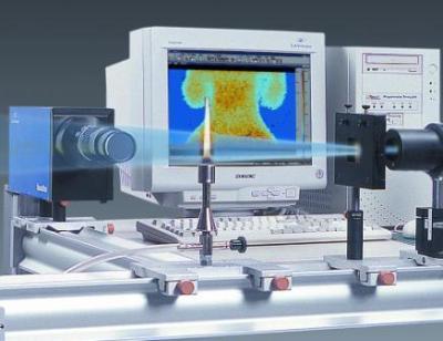
北京欧兰科技发展有限公司为您提供《内燃机中计算流体力学(CFD)分析检测方案(粒子图像测速)》,该方案主要用于汽车电子电器中其他检测,参考标准《暂无》,《内燃机中计算流体力学(CFD)分析检测方案(粒子图像测速)》用到的仪器有德国LaVision PIV/PLIF粒子成像测速场仪、LaVision SprayMaster 喷雾成像测量系统、汽车发动机多参量测试系统、PLIF平面激光诱导荧光火焰燃烧检测系统。
我要纠错
推荐专场


汽车尾气分析仪
更多


相关方案
 咨询
咨询