冲击射流中利用声作用力改善冲击射流热传导检测方案(粒子图像测速)

智能文字提取功能测试中

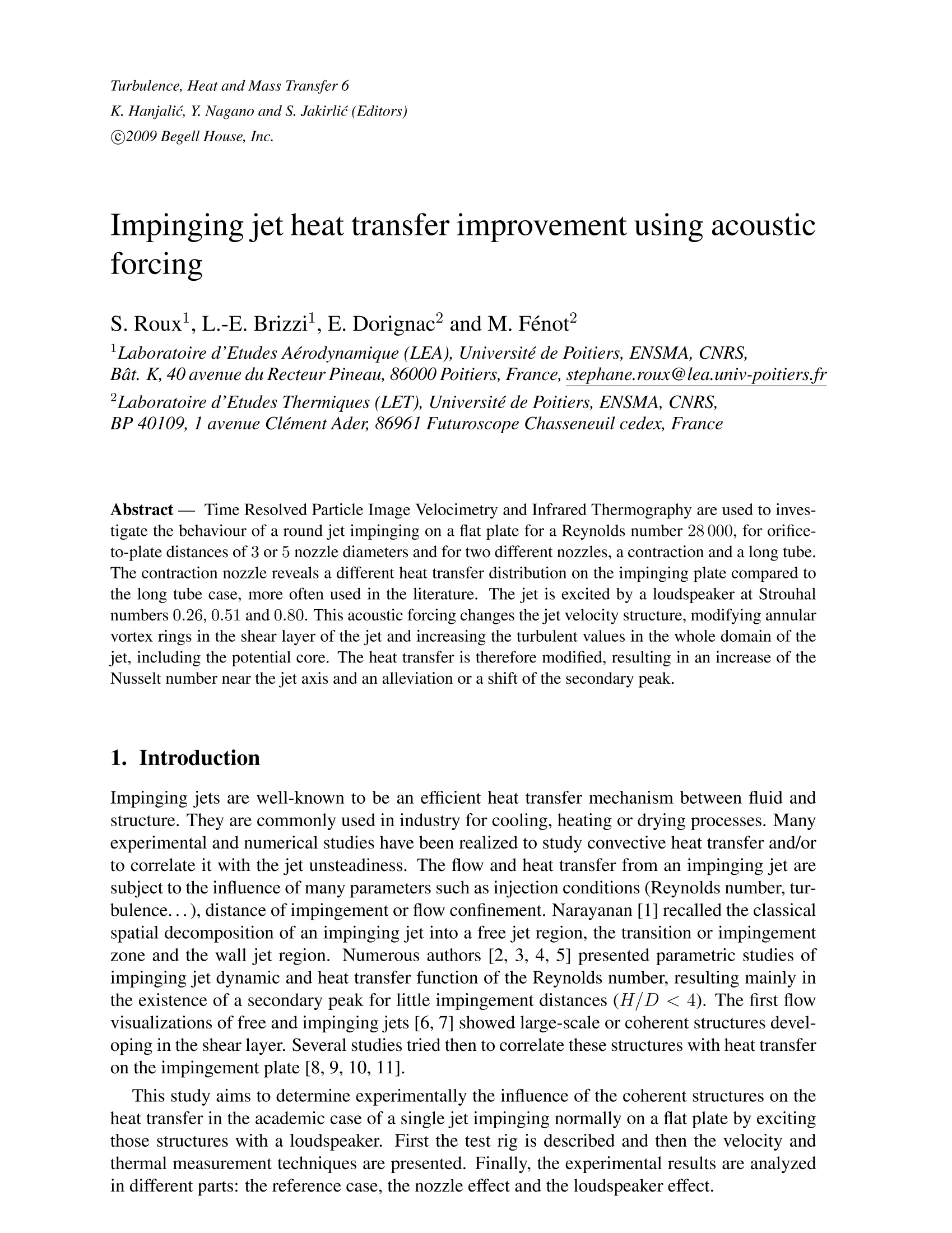
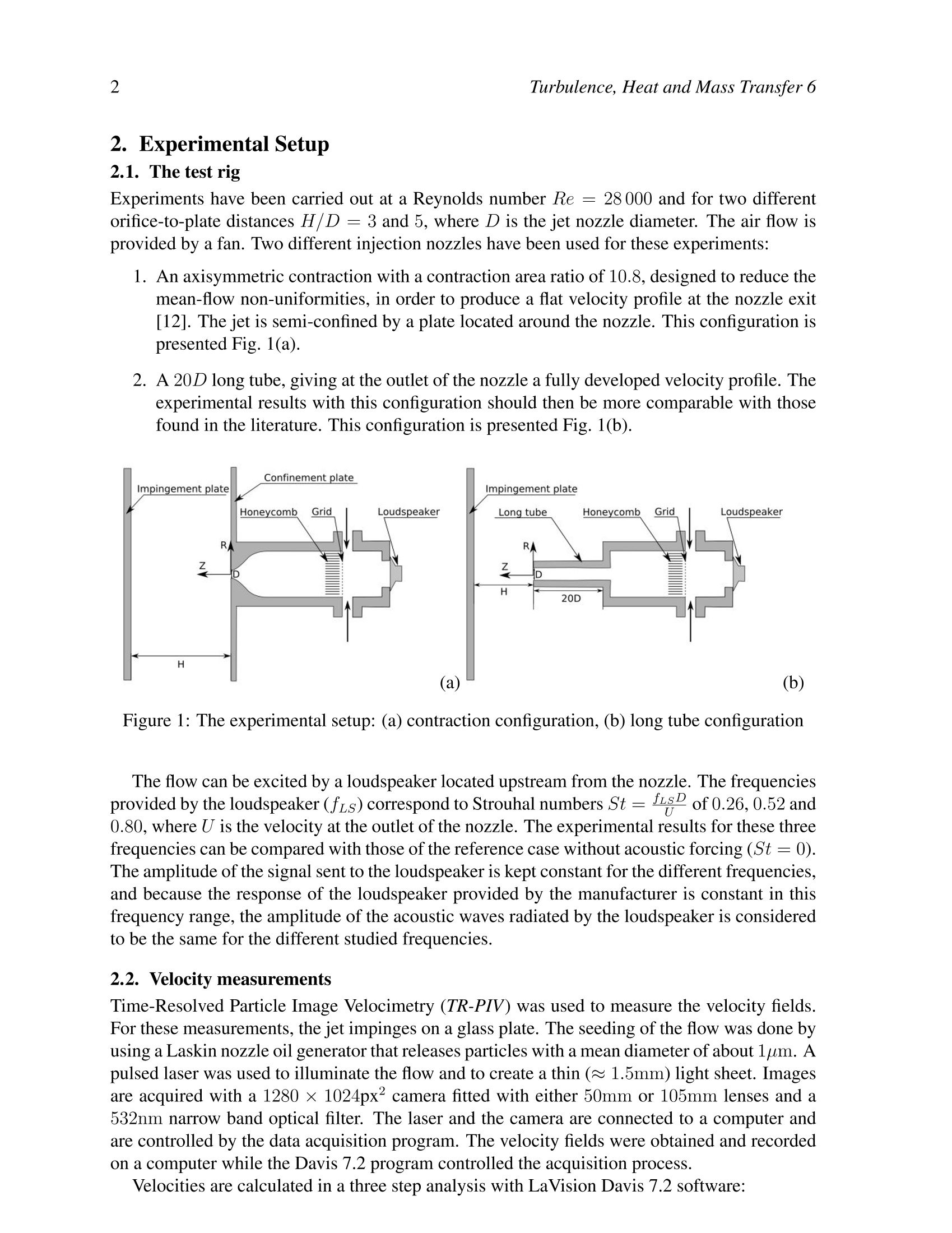
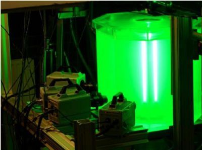
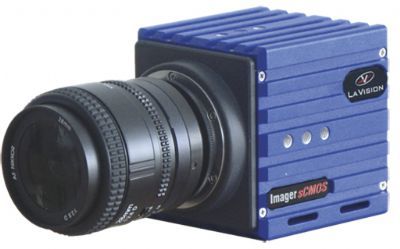
Turbulence， Heat and Mass Transfer 6K. Hanjalic， Y. Nagano and S. Jakirlic (Editors)C2009 Begell House， Inc. Turbulence， Heat and Mass Transfer 62 Impinging jet heat transfer improvement using acousticforcing S. Rouxl， L.-E. Brizzi， E. Dorignac’ and M. Fénot’ Laboratoire d'Etudes Aerodynamique (LEA)， Universite de Poitiers， ENSMA， CNRS， Bat. K， 40 avenue du Recteur Pineau， 86000 Poitiers， France， stephane.roux@lea.univ-poitiers.fr Laboratoire d'Etudes Thermiques (LET)， Universite de Poitiers， ENSMA， CNRS， BP 40109， I avenue Clement Ader， 86961 Futuroscope Chasseneuil cedex， France Abstract- Time Resolved Particle Image Velocimetry and Infrared Thermography are used to inves-tigate the behaviour of a round jet impinging on a flat plate for a Reynolds number 28 000， for orifice-to-plate distances of 3 or 5 nozzle diameters and for two different nozzles， a contraction and a long tube.The contraction nozzle reveals a different heat transfer distribution on the impinging plate compared tothe long tube case， more often used in the literature. The jet is excited by a loudspeaker at Strouhalnumbers 0.26， 0.51 and 0.80. This acoustic forcing changes the jet velocity structure， modifying annularvortex rings in the shear layer of the jet and increasing the turbulent values in the whole domain of thejet， including the potential core. The heat transfer is therefore modified， resulting in an increase of theNusselt number near the jet axis and an alleviation or a shift of the secondary peak. 1. Introduction Impinging jets are well-known to be an efficient heat transfer mechanism between fluid andstructure. They are commonly used in industry for cooling， heating or drying processes. Manyexperimental and numerical studies have been realized to study convective heat transfer and/orto correlate it with the jet unsteadiness. The flow and heat transfer from an impinging jet aresubject to the influence of many parameters such as injection conditions (Reynolds number， tur-bulence...)， distance of impingement or flow confinement. Narayanan [1] recalled the classicalspatial decomposition of an impinging jet into a free jet region， the transition or impingementzone and the wall jet region. Numerous authors [2， 3， 4， 5] presented parametric studies ofimpinging jet dynamic and heat transfer function of the Reynolds number， resulting mainly inthe existence of a secondary peak for little impingement distances (H/D <4). The first flowvisualizations of free and impinging jets [6， 7] showed large-scale or coherent structures devel-oping in the shear layer. Several studies tried then to correlate these structures with heat transferon the impingement plate [8，9，10， 11]. This study aims to determine experimentally the influence of the coherent structures on theheat transfer in the academic case of a single jet impinging normally on a flat plate by excitingthose structures with a loudspeaker. First the test rig is described and then the velocity andthermal measurement techniques are presented. Finally， the experimental results are analyzedin different parts： the reference case， the nozzle effect and the loudspeaker effect. 2. Experimental Setup 2.1. The test rig Experiments have been carried out at a Reynolds number Re = 28000 and for two differentorifice-to-plate distances H/D = 3 and 5， where D is the jet nozzle diameter. The air flow isprovided by a fan. Two different injection nozzles have been used for these experiments： 1. An axisymmetric contraction with a contraction area ratio of 10.8， designed to reduce themean-flow non-uniformities， in order to produce a flat velocity profile at the nozzle exit[12]. The jet is semi-confined by a plate located around the nozzle. This configuration ispresented Fig. 1(a). 2. A 20D long tube， giving at the outlet of the nozzle a fully developed velocity profile. Theexperimental results with this configuration should then be more comparable with thosefound in the literature. This configuration is presented Fig. 1(b). Figure 1： The experimental setup： (a) contraction configuration， (b) long tube configuration The flow can be excited by a loudspeaker located upstream from the nozzle. The frequenciesprovided by the loudspeaker (fLs) correspond to Strouhal numbers St=fusD of 0.26，0.52 and0.80， where U is the velocity at the outlet of the nozzle. The experimental results for these threefrequencies can be compared with those of the reference case without acoustic forcing (St=0).The amplitude of the signal sent to the loudspeaker is kept constant for the different frequencies，and because the response of the loudspeaker provided by the manufacturer is constant in thisfrequency range， the amplitude of the acoustic waves radiated by the loudspeaker is consideredto be the same for the different studied frequencies. 2.2. Velocity measurements Time-Resolved Particle Image Velocimetry (TR-PIV) was used to measure the velocity fields.For these measurements， the jet impinges on a glass plate. The seeding ofthe flow was done byusing a Laskin nozzle oil generator that releases particles with a mean diameter of about 1um. Apulsed laser was used to illuminate the flow and to create a thin (~1.5mm) light sheet. Imagesare acquired with a 1280 ×1024px’camera fitted with either 50mm or 105mm lenses and a532nm narrow band optical filter. The laser and the camera are connected to a computer andare controlled by the data acquisition program. The velocity fields were obtained and recordedon a computer while the Davis 7.2 program controlled the acquisition process. Velocities are calculated in a three step analysis with LaVision Davis 7.2 software： Image pre-processing： background image subtraction using the minimum value accordingthe time series. ·Correlation calculation： four step adaptive correlation (Initial pass 64 × 64， final pass16×16 doubled， 50% overlap) Spurious vectors detection： finally， validation steps are carried out in an effort to eliminateerroneous velocity vectors. The parameters， such as sampling frequency fs， number of measured velocity field N， spatialresolution， for each configuration are summed up in Tab. 1. The number of measured velocityfields ensures that the number of uncorrelated events was sufficient to get good statistics. Aminimum of 400 validated vectors were used in order to justify statistically the results that arepresented in this study. Finally，N 2D velocity fields with two components (ur，uz) are obtainedin a plane passing through the jet axis. Nozzle H/D fs(kHz) N Camera resolution (px) Spatial resolution (mm) Contraction 3 2 4000 892×876 Contraction 5 2 4000 1020 ×780 1.58 Long tube 3 1.5 2500 1018×1018 Table 1： TR-PIV parameters for the different configurations The errors inherent in the PIV measurements were quantified according to Westerweel [13]with a 95% confidence level. The errors of the method mainly depend on the scale calibration(≈ 0.65%)， the pixel displacement (≈ 1.04%) and the time interval between the two images(negligible uncertainty). To obtain the uncertainty of measurement， it is necessary to add to theprecision the various biases of this technique. There are many biases and some of them are noteasily quantifiable. For example， we can mention the bias related to interpolation sub-pixel[13]or the bias due to the zones with strong velocity gradient [14]. However if we assure that thebiases are less than twice of the uncertainty allotted to the precision， the uncertainty is estimatedat 3% for the mean values and at 6% for RMS. 2.3. Temperature measurements For thermal measurements， the jet impinges on an epoxy plate covered with a thin foil of copperon its front side. This foil is engraved by a circuit that is linked to a DC supply and allowsheating of the plate by Joule effect. The impingement plate is painted in black to have a highuniform emissivity (≈0.95) for precise radiative heat fluxes calculation and for thermographicmeasurement. An infrared camera (CEDIP Jade Irfpa) measures the backward temperature ofthe plate. In this study， which pertains to steady state， each thermographic image is the result ofthe mean of 500 images recorded during 10s. This average allows us to remove measurementnoise. The method used in this study to determine the heat transfer coefficient has been first de-scribed by Fenot et al. [15]. The general definition of heat transfer coefficient h， also known asNewton’s law of cooling is ： which can also be written by： where pco is the convective heat flux density on the front side， Tw is the front wall temperatureand Tref is the reference temperature depending on the configuration， and we searched a ref-erence temperature as heat transfer coefficient， which would be independant from the thermalconditions. So， for different flux densities， heat transfer coefficient h should remain the same.If four different convective heat flux densities are injected and if the wall temperature Tw ismeasured for each one， we should have a straight line linking each couple (Pco， Tw) as seen inFig.2(b). Then 1/h will be the slope and Tref the y-intercept. So， Tref is equal to the walltemperature when there is no exchange between the plate and the flow， which is precisely thedefinition of adiabatic wall temperature Tad. Moreover， using this definition， the heat transfercoefficient is assumed to be independent from flux density. If it is not， then the correlationcoefficient of linear regression will be far from 1. In practice， the technique consists in electrically heating the impingement plate using coppercircuits. This enables the experimenter to calculate the exact electrical flux density dissipatedby Joule effect pelec. Electrical resistivity variation with temperature is taken into account inthe calculation of heat fluxes. Radiative and convective losses must be calculated to obtain theconvective heat flux density on the front sidepco， which is an exchange between plate and jetsas presented in Fig. 2(a)： where pco，r is the convective heat flux density on the rear side， Prad，f is the radiative heat fluxdensity on the front side， Prad，r is the radiative heat flux density on the rear side， h， is the heattransfer coefficient on rear side， Tw，r is the rear wall temperature， T is the ambient temperature，Tinj is the injection wall temperature， o is the Stefan-Blotzman constant and ew is impingementwall rear side emissivity. Figure 2： The principle of thermal measurement postprocessing： (a) the heat fluxes， (b) the heattransfer determination Regarding the convective heat flux density on the rear side (co，r， a heat transfer coefficienth， has been measured when the jet is cut off. As the impinging plate is located vertically(with gravity along theY axis)， h， varies according to Y. Radial heat conduction within theimpingement wall can be overlooked due to the relatively homogenous temperature of the plate.Temperature is measured at the rear side of the plate and Tu can be deduced from Tw，r with： where e is the impingement plate thickness and is the wall thermal conductivity. Local heattransfer coefficient h is made dimensionless with Nu=hD， where the air thermal conductivityair is calculated for the adiabatic temperature Tad· Uncertainties are estimated using a statistical approach. Taking into account errors due toambient and injection temperature， to electrical， radiative and convective fluxes， and to emis-sivities， random uncertainty for the Nusselt number values is no higher than 5%. Overall uncer-tainty does not exceed 12%. All these uncertainty values have been reported at a 95% confidencelevel. 3. Results 3.1. Reference case Velocity and thermal results are presented for the reference case， without acoustic forcing (St =0)， for the two orifice-to-plate distances (H/D=3 and 5) and with the contraction nozzle. Fig.3 shows instantaneous， mean and root-mean-squared velocity fields in this configurationfor the two orifice-to-plate distances. The jet can typically be split into three regions [1]： First，a free jet region， at the outlet of the nozzle， where the flow is not significantly influenced by theimpinging plate. The main component of the velocity is axial (uz). The jet is then developinguntil Z/D=2 in the H/D=3 case and until Z/D=4 in the H/D=5 case. The jet is thendiverted in the impinging or transition zone. In this region， the jet has initially an axial mainvelocity component which converts to a radial mean velocity component， along the impinging Figure 3： Normalized velocity fields with the contraction nozzle without acoustic forcing：H/D =3： (a) instantaneous u， (b) mean u， (c) RMS u'ms. H/D= 5： (d) instantaneousu， (e) mean u， (f) RMS urms. plate. In both cases， this area is located for |R|/D <2. Finally a wall jet region for|R|/D> 2，where the main velocity component is radial (ur) and the boundary layer thickness increasesradially. The potential core of the jet extends to Z/D= 4 in the H/D= 5 case and impingesthe plate for H/D=3. The turbulent statistical velocities (urms) are located exclusively in theshear layer and in the wall jet. On Fig. 4， the radial variations of Nusselt number are represented for the two orifice-to-platedistances. For H/D = 5， the secondary peak is not present as it was expected， whereas it islocated around R/D= 2 in the H/D =3 case. Moreover， for H/D=3， the jet axis doesnot coincide with a maximum heat transfer. This might be explained by the shape of the nozzlewhich is here a contraction and gives a flat velocity profile， whereas a long tube is more oftenused in literature， which gives a parabolic profile. More comments about this will be given insection 3.2. Figure 4： Normalized heat transfer coefficient h with the contraction nozzle without acousticforcing. 3.2. Nozzle effect The results without acoustic forcing for the two orifice-to-plate distances and for the two differ-ent nozzles are compared in this section. Fig. 5 compares the mean velocity profiles for the twonozzles for H/D= 3 at Z/D=0.15. As expected， for the contraction， the velocity profile isflat， whereas it has a parabolic shape for the long tube. Figure 5： Mean normalized velocity profiles for the long tube and the contraction nozzle forH/D= 3 at Z/D=0.15. Fig. 3 for the contraction and Fig. 6 for the long tube show instantaneous and statisticalvelocity fields. The decomposition into three regions is not significantly modified： the free jetregion until Z/D= 2 for H/D=3 and Z/D= 4 for H/D=5， then the transition zone for|R|/D <2 and finally the wall jet region for|R|/D>2. The turbulence levels are comparablein the shear layer and in the wall jet. However， near the stagnation point， whereas the turbulencelevels are very low and near zero for the contraction， they are higher and significant in the longtube configuration. Figure 6： Normalized velocity fields with the long tube without acoustic forcing： H/D=3：(a) instantaneous u， (b) mean u， (c) RMS ums. H/D= 5： (d) instantaneous u， (e) mean u， (f)RMS urms. Fig. 7(a) and (b) compare the radial variations of the Nusselt number for the two nozzlesfor H/D = 3 (Fig. 7(a)) and H/D= 5 (Fig. 7(b)). For H/D =5， the radial evolutions ofthe Nusselt number are quite similar. Nusselt number is higher in the long tube configuration，which can be explained by the slightly higher turbulence levels at the impinging plate， especiallynear the stagnation point. For H/D=3， the radial variations of the Nusselt number are verydifferent. First， with the long tube， the jet axis coincides with a maximum of heat transfer. Figure 7： Normalized heat transfer coefficient h with different nozzles without acoustic forcing：(a) H/D=3，(b)H/D=5. This maximum is due to the parabolic velocity profile， more often used in literature. With thecontraction， the maximum occurs around R/D= 0.5， where the jet shear layer impinges theplate. Near the jet axis， turbulent levels are very low， which could explain the loss of heattransfer at the stagnation point. The higher turbulent levels with the long tube could explain thehigher Nusselt number for R/D <1. Then， the characteristic secondary peak is shifted betweenthe two configurations： with the contraction， it is located around R/D=2， whereas it is aroundR/D=2.4 with the long tube. This difference could be explained by the development of thewall jet. With the contraction， the wall jet boundary layer seems to begin expanding aroundR/D=2， whereas with the long tube， it does not expand at the limit of the PIV window. Moreprecise measurements at the impingement plate are required to confirm that. 3.3. Loudspeaker effect Fig. 8 represents instantaneous， mean and RMS velocity fields for the two orifice-to-plate dis-tances， with the contraction and with an acoustic forcing at St = 0.26. The forcing Strouhalnumber is near the Strouhal number of the natural oscillation of a free jet (St =0.3， [6]). Aresonance phenomenon is then shown： the acoustic forcing creates large annular vortex rings atthe nozzle lip in the jet shear layer. That implies several changes in the statistical velocity fields.First， in the mean velocity field， the shear layer does not increase linearly as in the referencecase. Indeed， the vortices production implies a fast increase of the jet diameter at the nozzleoutlet， then the jet diameter remains constant until the impingement plate begins to have an ef-fect. The turbulent statistical fields are very different than in the reference case： they are locatedall over the jet domain (there is no more potential core) and not only in the shear layer. Theturbulent intensity is around three times greater for H/D= 5 and twice greater for H/D=3.For H/D = 5， a zone with very low velocities is between two consecutive structures， whichexplains these very high turbulent levels. The structures are less noticeable in the H/D = 3case， which could be explained by a blockade effect due to the relatively low orifice-to-platedistance. The vortex rings are very stable and impinge the plate and propagate in the radialdirection. Figure 8： Normalized velocity fields with the contraction nozzle with acoustic forcing at St =0.26： H/D=3： (a) instantaneous u， (b) mean u， (c) RMS urms.H/D=5： (d) instantaneousu， (e) meanu， (f) RMS ums. Fig. 9 represents instantaneous， mean and RMS velocity fields for the two orifice-to-platedistances， with the contraction and with an acoustic forcing at St =0.52. The jet structure ismore classical， the turbulent quantities have higher values， but remain comparable to those ofthe reference case. The acoustic forcing creates also annular vortex rings， but at a frequencytwice higher than in the last case. Two consecutive vortex rings can sometimes pair near theimpingement plate for H/D=5， forming a larger vortex ring at a Strouhal number St =0.26，near the Strouhal number of the natural oscillation of a free jet. The blockade effect is alsoshown for H/D =3， for the structures are less intense than in the H/D = 5 case. Turbulentstatistics are then also slightly lower. Figure 9： Normalized velocity fields with the contraction nozzle with acoustic forcing at St=0.52： H/D=3： (a) instantaneous u，(b) mean u， (c) RMS urms. H/D=5： (d) instantaneousu， (e) mean u， (f)RMS u ms Fig. 10 represents instantaneous， mean and RMS velocity fields for the two orifice-to-platedistances， with the contraction and with an acoustic forcing at St =0.80. For H/D = 3，the instantaneous and statistical velocity field are very similar to those found with an acousticforcing at St =0.52. For H/D = 5， two consecutive vortex rings always pair at the samelocation Z/D= 2. This explains the original shapes of the mean and turbulent velocity fields：the mean velocity field shows a strewing of the jet near the location of the pairing. The turbulentvelocity field urms is similar to the one found for St =0.52， then the values increase in thepotential core and in the shear layer. This can be explained by the second vortex ring of thepairing coming into the first one， creating more unsteadiness. Then， there is only one vortex ringleft， and the velocity fields are again similar to those found with St = 0.52. It is also importantto notice that in the H/D = 3 case， a pairing phenomenon also begins when the structures reachZ/D=2. However， because of the impingement， the first vortex ring is diverted to the radialdirection before the second one could come into the first. So this phenomenon rarely ends to apairing of the two vortex rings. Figure 10： Normalized velocity fields with the contraction nozzle with acoustic forcing at St =0.80： H/D=3： (a) instantaneous u， (b) mean u， (c) RMS ums.H/D=5： (d) instantaneousu， (e) mean u， (f) RMS urms. On Fig. 11， the radial variations of Nusselt number for different acoustic forcing Strouhalnumbers for H/D = 5 are represented. The acoustic forcing does not seem to have a strongeffect on the heat transfer， probably because the large annular vortex rings， considered as coher-ent structures， stay far enough from the impingement plate， so that they have less effect on theheat transfers. Indeed， the rings are diverted from the free jet zone to the wall jet region withoutimpinging directly the plate. The Nusselt number is higher near the jet axis with forcing，whichcan be explained by the higher turbulent levels with acoustic forcing. 4 Figure 11： Normalized heat transfer coefficient h with the contraction nozzle with differentacoustic forcing Strouhal numbers for H/D=5. On Fig. 12， the radial variations of Nusselt number for different acoustic forcing Strouhalnumbers for H/D= 3 are represented. The Nusselt number distributions are very different foreach acoustic forcing Strouhal number. First， for St=0.26， the Nusselt number is higher near the jet axis. This can be explained bythe higher turbulence levels. The first peak， due to the contraction nozzle， is less important thanin the reference case， probably because of the unsteadiness of the forced jet. The secondary peak， clear in the reference case， is totally removed with this acoustic forcing. Then， for St =0.52， the main difference with the reference case is that the secondary peakseems to be shifted from R/D=2 in the reference case to R/D=1.6. This may be linked tothe fact that the wall jet seems to begin its spreading around this location. Again， more precisemeasurements at the impingement plate are required to confirm that. Close to the jet axis， theNusselt number is almost the same in both cases， as the turbulent intensities are comparable. Finally， for St=0.80， the Nusselt number is higher near the jet axis， as turbulent intensities.The inner vortex ring of the failed pairing phenomenon could also have an effect on that， forit impinges on the plate near the jet axis， and is diverted very late. As in the St=0.52 case，the secondary peak is only a change of curvature and not a real peak， and is shifted aroundR/D=1.6. 4 Figure 12： Normalized heat transfer coefficient h with the contraction nozzle with differentacoustic forcing Strouhal numbers for H/D=3. 4. Conclusion A round jet impinging on a flat plate and forced by a loudspeaker has been experimentallystudied using Time Resolved Particle Image Velocimetry and Infrared Thermography. The longtube configuration permits to compare the results with the literature. The use of a contractioninstead of a long tube has several effects on the heat transfer， especially near the jet axis. Theacoustic forcing can radically change the flow structure， creating annular vortex rings in theshear layer of the jet， considered as coherent structures. Pairing phenomenon takes place in thejet for higher and non-natural Strouhal number forcing. This acoustic forcing has not a strongeffect on the heat transfer for H/D = 5， however for H/D=3， the forcing can modify theNusselt number distributions. The secondary peak， which is clearly detected without forcing，seems to have been shifted or alleviated with acoustic forcing. These results give another evi-dence that the large scale turbulent structures have a strong effect on the heat transfer coefficienton the impinging plate for little orifice to plate distances. References 1. V.Narayanan，J. Seyed-Yagoobi， and R.H. Page. An experimental study of fluid mechanicsand heat transfer in an impinging slot jet flow. International Journal of Heat and MassTransfer， 47：1827-1845，2004. 2. M. Fairweather and G.K. Hargrave. Experimental investigation of an axisymmetric， im-pinging turbulent jet. 1. velocity field. Experiments in Fluids， 33：464-471，2002. 3. M. Fairweather and G.K. Hargrave. Experimental investigation of an axisymmetric， im-pinging turbulent jet.2. scalar field. Experiments in Fluids， 33：539-544， 2002. 4. D. Cooper， D.C. Jackson， B.E. Launder， and G.X. Liao. Impinging jet studies for tur-bulence model assessment-i. flow-field experiments. International Journal of Heat andMass Transfer， 36：2675-2684，1993. 5. T.S.O’Donovan and D.B. Murray. Jet impingement heat transfer -part i： mean and root-mean-square heat transfer and velocity distributions. International Journal of Heat andMass Transfer， 50：3291-3301，2007. 6. S.C. Crow and F.H. Champagne. Orderly structure in jet turbulence. Journal of FluidMechanics，48：547-591，1971. 7. C.O. Popiel and O. Trass. Visualization of a free and impinging round jet. ExperimentalThermal and Fluid Science， 4：253-264，1991. 8.T.S. O'Donovan and D.B. Murray. Jet impingement heat transfer - part ii： a temporalinvestigation of heat transfer and local fluid velocities. International Journal of Heat andMass Transfer， 50：3302-3314，2007. 9. M. Hadziabic and K. Hanjalic. Vortical structures and heat transfer in a round impingingjet. Journal of Fluid Mechanics， 596：221-260， 2008. 10. J.W. Hall and D. Ewing. On the dynamics of the large-scale structures in round impingingjets. Journal of Fluid Mechanics， 555：439-458，2006. 11. J. Vejrazka. Experimental study ofa pulsating round impinging jet. PhD thesis， InstitutNational Polytechnique de Grenoble，2002. 12. T. Morel. Comprehensive design of axisymmetric wind tunnel contractions. Journal ofFluids Engineering， pages 225-233， June 1975. 13. J. Westerweel. Theoritical analysis of the measurement precision in particle image ve-locimetry. Experiments in Fluids， Suppl.：S3-S12， 2000. 14. R. D. Keane and R. J. Adrian. Optimization of particle image velocimeters. part i： Doublepulsed systems. Meas. Sci. Technol.，1：1202-1215，1990. 15. M. Fenot， J.-J. Vullierme， and E. Dorignac. A heat transfer measurement of jet impinge-ment with high injection temperature. C. R. Mecanique， 333：778-782， 2004.