方案详情文
智能文字提取功能测试中
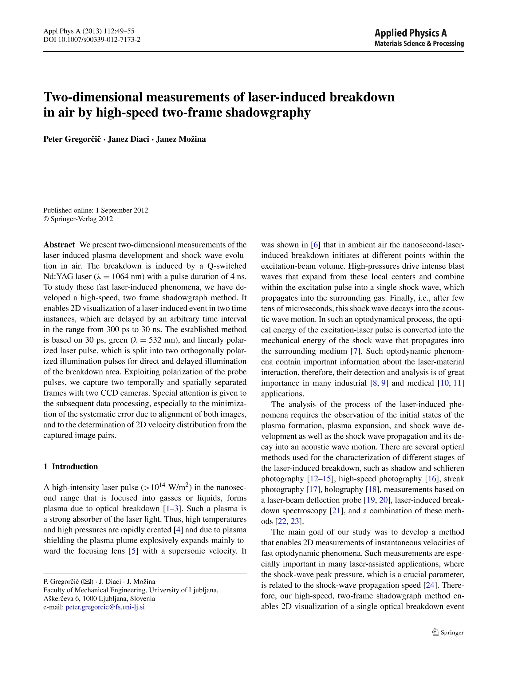
Applied Physics AAppl Phys A (2013) 112:49-55DOI 10.1007/s00339-012-7173-2Materials Science & Processing P. Gregorcic et al.50 Two-dimensional measurements of laser-induced breakdownin air by high-speed two-frame shadowgraphy Peter Gregorcic.Janez Diaci · Janez Mozina Abstract We present two-dimensional measurements of thelaser-induced plasma development and shock wave evolu-tion in air. The breakdown is induced by a Q-switchedNd:YAG laser (=1064 nm) with a pulse duration of 4 nsTo study these fast laser-induced phenomena, we have de-veloped a high-speed, two frame shadowgraph method. Itenables 2D visualization of a laser-induced event in two timeinstances, which are delayed by an arbitrary time intervalin the range from 300 ps to 30 ns. The established methodis based on 30 ps, green (= 532 nm), and linearly polar-ized laser pulse, which is split into two orthogonally polar-ized illumination pulses for direct and delayed illuminationof the breakdown area. Exploiting polarization of the probepulses, we capture two temporally and spatially separatedframes with two CCD cameras. Special attention is given tcthe subsequent data processing, especially to the minimiza-tion of the systematic error due to alignment of both images,and to the determination of 2D velocity distribution from thecaptured image pairs. 1 Introduction A high-intensity laser pulse (>1014 W/m²) in the nanosec-ond range that is focused into gasses or liquids, formsplasma due to optical breakdown [1-3]. Such a plasma isa strong absorber of the laser light. Thus, high temperaturesand high pressures are rapidly created [4] and due to plasmashielding the plasma plume explosively expands mainly to-ward the focusing lens [5] with a supersonic velocity. It ( P.Gregoric(区)·J.Diaci · J. MozinaFaculty of Mechanical Engineering, University of Ljubljana,Askerceva 6, 1000 Ljubljana, Slovenia e-mail: p ete r .g re go rcic@fs.uni- l j. s i ) was shown in [6] that in ambient air the nanosecond-laser-induced breakdown initiates at different points within theexcitation-beam volume. High-pressures drive intense blastwaves that expand from these local centers and combinewithin the excitation pulse into a single shock wave, whichpropagates into the surrounding gas. Finally, i.e., after fewtens of microseconds, this shock wave decays into the acous-tic wave motion. In such an optodynamical process, the opti-cal energy of the excitation-laser pulse is converted into themechanical energy of the shock wave that propagates intothe surrounding medium [7]. Such optodynamic phenom-ena contain important information about the laser-materialinteraction, therefore, their detection and analysis is of greatimportance in many industrial [8,9] and medical [10, 11]applications. The analysis of the process of the laser-induced phe-nomena requires the observation of the initial states of theplasma formation, plasma expansion, and shock wave de-velopment as well as the shock wave propagation and its de-cay into an acoustic wave motion. There are several opticalmethods used for the characterization of different stages ofthe laser-induced breakdown, such as shadow and schlierenphotography [12-15], high-speed photography [16], streakphotography [17], holography [18], measurements based ona laser-beam deflection probe [19, 20], laser-induced break-down spectroscopy [21], and a combination of these meth-ods [22,23]. The main goal of our study was to develop a methodthat enables 2D measurements of instantaneous velocities offast optodynamic phenomena. Such measurements are espe-cially important in many laser-assisted applications,wherethe shock-wave peak pressure, which is a crucial parameter,is related to the shock-wave propagation speed [24]. There-fore, our high-speed, two-frame shadowgraph method en-ables 2D visualization of a single optical breakdown event in two time instances [6]. The method is based on 30-ps,linearly polarized pulse, which is split into two orthogonallypolarized probe pulses for the direct and delayed illumina-tion of the breakdown area. Using an optical delay line, avariable delay between the direct and the delayed illumina-tion can be achieved in the range between 300 ps and 30 ns.The established method presents an accessible solution formany industrial and medical research environments, wheretemporally and spatially observation of different kinds oflaser-induced phenomena in all kinds of transparent mediais required. In this contribution, we describe the developed shad-owgraph method and subsequent data processing based onthe analysis of image pairs acquired during a single break-down event. Such an analysis allows the determination of2D velocity fields of the breakdown area. We show that ourmethod enables the shadowgraphic observation of all stagesof laser-induced breakdown including the breakdown initi-ation and plasma development within the irradiation withthe excitation-laser pulse. The main focus of the presentedexperiments are the 2D measurements of instantaneous ve-locities of plasma and shock-wave evolution in air from thevery beginning of the laser-induced breakdown to the times,when the shock wave decays into an acoustic wave. By wayof these measurements, we demonstrate and discuss the ca-pability of the presented shadowgraph method. 2 Experimental setup The top view of our high-speed, two-frame shadowgraphmethod for observation of the laser-induced breakdown isschematically shown in Fig. 1. The breakdown in ambientair is induced by a Q-switched Nd: YAG laser (X=1064 nm, Quantel, France, Brio) employed as the excitation source. Itemits 4-ns (FWHM) pulses with energy EL=12.7 mJ±0.5 mJ and peak power PL =2.9 MW ±0.5 MW afterthe attenuator (A). Since the excitation beam is partially re-flected by the polarizer inside the attenuator, its energy canbe simultaneously measured by the energy meter (E) duringthe experiments. After the attenuator, the excitation beamis guided through the beam expander (BE) and focused bythe lens (L) with a focal length of 120 mm to a diameter of25 um in air. Thus, in the focus, it achieves the peak inten-sity around6×1015W/m², which is just above the thresholdintensity. i.e., Ith ~5×10¹⁵ W/m2. The laser-induced breakdown in air is examined usinghigh-speed, two-frame shadowgraphy. Here, a frequency-doubled Nd:YAG laser (Ekspla, Lithuania, PL2250-SH-TH) emitting green (入=532nm) pulses with duration of30 ps (FWHM) is used as an illumination source. Afterthe half-wave plate (HWP), the illumination-beam polar-ization forms a 45° angle with respect to the optical table.The first polarizing beam splitter (PBS) is used to dividethe single illumination-pulse into two pulses with perpen-dicular linear polarizations. The x-polarized pulse (the di-rect probe) hits the breakdown area directly, while the y-polarized pulse (the delayed probe) passes an optical delayline before hitting the breakdown area. By using the secondPBS, both probe-pulses illuminate the breakdown regionalong the same path. Before the breakdown area, the probesare expanded with the BE. A narrow band-pass filter (BPF)centered at 532 nm ±10 nm is placed between the break-down region and the microscope to block the light emittedfrom plasma. Another PBS is placed inside the microscope,where it transmits the direct (x-polarized) probe to the CCDcamera Cx and reflects the delayed (y-polarized) probe tothe CCD camera Cy. In such a way, we use the polariza-tion of both probes to capture two temporally and spatially Fig. 1 Schematic top view ofthe high-speed, two-frameshadowgraphy separated frames with two CCD cameras (Basler AG, Ger-many, scA1400-17fm, 1.4 Mpx). The spatial resolution ofour optical system is in the range of K=0.7-1.5 um/px. Fora particular series of measurements,k value was determinedusing images of a calibrating pattern. The probe pulses are delayed by an optical delay line. Inour case, the path of the delayed probe is 0.1-10 m longerthan the path of the direct probe. Therefore, we can producean arbitrary time delay, At, between the probes in the rangefrom 300 ps to 30 ns. Here, the shortest time delay, At, istheoretically limited by the illumination-pulse duration, butpractically it should be at least 1 order of magnitude longer.On the other hand, the longest time delay between probe-pulses is limited by the stability of the optical components inthe delay line. Since the accuracy of the path of the delay lineis around 1 mm, the uncertainty of the time delay betweenboth probes is less than 10 ps. The lasers and cameras are synchronized with a signalgenerator (SG) connected to a personal computer. Therefore,the time delay, t1, between the illumination and excitationsource is defined by an electric delay produced by the SG.This delay between lasers has been chosen in the range from10 ns to 20 us in steps of 1 ns. Resolution down to 100 pshas been achieved by repeated measurements exploiting jit-ter of this synchronization, which is ±6 ns. The illumination and excitation pulses are partially re-flected by dielectric plates to the fast photodiodes PDi andPDe, respectively. The used photodiodes with a bandwidthof 1 GHz have a rise time of 600 ps. Assuming that thecoaxial cables from both photodiodes to the oscilloscope(LeCroy, US, 600 MHz Wave Runner64MXi-A, a samplingrate of 10 GS/s) are of equal length, the time delay, t1, be-tween the direct-probe pulse and the excitation pulse at thebreakdown region can be calculated as Here, AtpD stands for the delay between the signals ac-quired from PDi and PDe; di1, dei are the distances between the dielectric plates and photodiodes PDi and PDe, respec-tively; di2, de2 are the distances between the dielectric platesand the breakdown region (see Fig. 1); and c is the speed oflight in the air. Time t corresponds to the time of directlyexposed image captured by camera Cx, while the time of thedelayed exposure t2, captured by camera Cy, can be calcu-lated as t2=t1+At. The experimental setup is controlled with custom devel-oped software that enables the data acquisition from a digitaloscilloscope and subsequent signal processing as well as theimage acquisition from cameras. In the offline processing,this software is also used for the subpixel alignment of cap-tured images and subsequent image processing, described inthe next section. 3 Data processing The measurements of the optical breakdown by the de-scribed method are based on the image pairs, which are ac-quired during a single breakdown event. The shutters of thetwo cameras are open during the measurements, while two.....30-ps-long illumination pulses hit the breakdown region attimes t and t2. An example of such image pair is shownin Fig. 3a. Since typical pairs of images captured by differ-ent time delays, At, are presented in detail in our previouswork [6], we will restrict ourselves here to the description ofdata processing. Here, the main emphasis is given to (i) theminimization of the systematic error due to alignment ofboth images; and (ii) the determination of 2D velocity dis-tribution from captured image pairs. 3.1 Image pair alignment Before the measurements, the cameras are mechanicallyaligned. A typical image pair showing the alignment of cam-eras is presented in Fig. 2a. Here, we use the setup sketchedin Fig. 1, where the cross-pattern printed on a paper is placed Fig. 2 Software alignment ofimage pairs. (a) Thecross-pattern captured by bothcameras after the mechanicalalignment. (b) Thedetermination of thecross-pattern captured by Cx(the blue dots) and Cy (the reddots). The fitted linear functionsto these dots (the broken lines)are used to obtain the spatialtransformation of image fromCy Fig. 3 The procedure for determination of 2D velocity distribution.(a) Typical image pair showing the shock wave at times t and t2. Thesolid lines show Bezier splines, while the control points are markedwith the white points. (b)The boundaries of the shock wave captured in the breakdown region and illuminated by a light from thefront side. The comparison between images from Cx and Cyin Fig. 2a reveals that the same pattern is placed at differ-ent positions in the images. Therefore, one of both imagesshould be software-aligned (translated and rotated) duringdata processing to avoid the systematic error of calculatedvelocities. To do this, we first use the image processing todetermine the cross-pattern captured by Cx (the blue dots inFig. 2b) and Cy (the red dots in Fig. 2b). Then the linearfunctions are fitted to dots representing the horizontal (thefull line in Fig. 2a) and vertical (the broken line in Fig. 2a)lines of this pattern. The fitted linear functions are shownas broken lines in Fig. 2b. From the intersections and theslopes of these functions, we determine the spatial transfor-mation (translation and rotation). Using this transformation,we transform the image from Cy by a bilinear interpolationalgorithm so that it is aligned with the image from Cx witha subpixel accuracy. 3.2 Determination of 2D velocity distribution The2D velocity distribution is calculated from shock waveboundaries in the image pair. The procedure for determina-tion of the 2D velocity distribution is presented in Fig. 3.Figure 3a shows a typical image pair captured at t1=12.6 nswith the optical delay between probe pulses △t =11.2 ns.The shape of the shock wave is first approximated by aBezier spline [25],i.e., a series of cubic Bezier curves joinedend to end in the control points. The control points (the whitepoints in Fig. 3a) are manually selected so that the Bezierspline (the blue and the red line in Fig. 3a) coincides withthe shape of the shock wave. by Cx (the blue points) and Cy (the red points). The green points showthe position of the calculated velocities. (c) Determination of the dis-tance ▲d;.(d) Calculated velocities for each point P; In Fig. 3b, the blue points correspond to the boundaryof the shock wave captured with the Cx, while the redpoints represents the spline showing the shock wave cap-tured t = 11.2 ns later with the Cy. For each point, Pi,at the boundary of the Cx (the blue points in Fig. 3b), thevelocity u; is calculated as In Eq. (2), i stands for the index of each point, the distanceAdi equals the shift (in pixels) of the point Pi during thetime interval At, and k is the spatial resolution of the opticalsystem. The shift Ad; is determined from the captured images asis shown in Fig. 3c. First, the normal to the spline at thepoint Pi=(xp,yP) is calculated.The corresponding pointQi=(xg;,yoi) at the Cy is determined as the intersectionbetween this normal and the spline describing the shape ofthe shock wave captured at t2. The distance (in pixels) be-tween points Piand Qi is calculated as while the time t and the position di of the calculated velocityui are determined as After the above procedure, we have the position of the shockwave boundary at time t (the green points in Fig. 3b) and the2D distribution of its velocities. The calculated velocities foreach point Pi are presented in Fig. 3d. Fig. 4 2D velocity distribution.(a) The shapes of the shockwaves at selected times t. Theshock waves have aligned thegeometric centers. (b) Thevelocity as a function of angle,defined in (a) b Angle [] The described data processing was used to obtain 2D veloc-ity distribution of the shock wave propagation at differenttimes t. The measured velocities for selected times are pre-sented in Fig. 4. Figure 4a shows the shapes of the shockwave at t={2.9 ns,5.3 ns, 9.8 ns,18.3 ns, 44.2 ns, 76.6 ns,125 ns}, where t = 2.9 ns corresponds to the innermostshock wave. In order to show the calculated velocity as afunction of angle, the geometric centers of shock waves inFig. 4a are manually aligned. Dimensions of the CCD sensorlimit the maximum dimension of the captured phenomenonat a particular spatial resolution k. For this reason, the k val-ues have been increased from 0.7 um/px for the innermostto 1.5 um/px for the outermost shock wave in Fig. 4a. Figure 4b shows the velocities of each measured shockwave as a function of angle (defined in Fig. 4a). Here, the90° angle corresponds to the top of the shock wave, i.e., itspart that propagates toward the excitation laser. Vice versa,the -90° angle corresponds to the bottom of the shock wave,which propagates away from the excitation laser. Immedi-ately after the breakdown, the top and the bottom of theshock wave have much higher velocities than its left andright side. This results in the ellipsoidal shape. It can beseen from Fig. 4b that the bottom has lower velocity duringthe excitation-laser radiation (t <10 ns) due to strong ab-sorption of the laser light in the plasma, resulting in plasmashielding. The velocity peaks at ±90°disappear after theend of the excitation pulse. Moreover, the velocities of thesepeaks at t = 18.3 ns are lower than the velocities in the hori-zontal directions (0° and 180°). Due to this reason, the ellip-soidal shock wave converts into a shock wave with a spheri-cal shape. More than 100 ns after the breakdown the velocityas a function of angle is approximately constant as it is evi-dent from the bottom two curves in Fig. 4b. In order to present the capabilities and limitations of thedeveloped method, we have measured the axial velocitiestoward the focusing lens (i.e., the velocities at angle 90°in Fig. 4). These velocities as a function of time are pre-sented in a log-log plot in Fig.5. Here, the inset shows the Fig.5 Axial velocity of the shock wave development toward the ex-citation laser as a function of time t. The green solid curve is the fit ofEq. (5) to the data measured at times t >t. The inset shows the powerof an excitation-laser beam as a function of time power of the excitation pulse versus time and the time zerocorresponds to the triggered value of the excitation-pulsepower. From the inset in Fig.5, it can be estimated that thepower threshold in our case is around Pth ~2.6 MW. Forour spot size, this matches the intensity threshold aroundIth ~5×10¹⁵ W/m², which is in agreement with valueslisted in the literature [3, 26]. The shaded area in Fig. 5as well as in the inset shows the time interval during theexcitation-laser radiation. Within the first two nanoseconds after the breakdowninitiation (i.e., in the time interval from t ~ 2.5 ns tot ~5 ns), the measured axial velocities of the edge of theplasma plume vary from 600 km/s to 100 km/s, which con-forms with the ionization front velocities presented else-where [4]. Here, a significant measurement noise (the bluepoints in Fig. 5) arises from the different mechanisms ofplasma expansion [4, 5]. The higher velocities (i.e., greaterthan 250 km/s) are recorded during fast ionization, whilethe lower axial velocities are related to the events cap-tured during the laser-supported detonation wave. When theexcitation-pulse power becomes too low to allow air ioniza- tion (t > 5 ns), the fast ionization phase ends and the mea-surement noise in Fig. 5 is significantly reduced. However,the shock wave is still plasma-driven and its shape is ellip-soidal (see Fig. 4a), as has been already shown by many au-thors (e.g., see [8,27]). In the time interval from t ~5 nsto t ~10 ns, the plasma energy still increases due to the ab-sorption of the laser-radiation. When the excitation-laser ra-diation ends (t > 10 ns), the high-temperature plasma drivesthe shock wave, thus prolonging its explosive expansion.This ends at ts =36 ns, when the shock wave energy be-comes constant (if the energy dissipation is negligible) andthe ellipsoidal shape of the shock wave is converted intoa nearly spherical shape, as can be seen in Fig. 4a (seealso[27]). The Jones theory for the intermediate strength blastwave [24] can be employed to describe propagation of theshock wave past ts. The solid line in Fig. 5 represents thefitted theoretical velocity derived from the model for thespherical blast wave [24]: u(t; Eo,to) Here, the energy of the shock wave Eo and the time offset toare the fitting parameters. In Eq. (5), the po is the ambientpressure, y=1.4 is the specific-heat ratio, 入5=1.175 is adimensionless geometry-dependent parameter [28, 29], andco =346 m/s is the speed of sound in air for the ambientconditions (po=10 Pa, To=25℃). Equation (5) is valid for the point explosion, where thewhole energy is released at once at time t=0. In our case,the energy of the shock wave increases during the plasmaexpansion. This is the reason that we have added an addi-tional fitting parameter, to into Eq. (5). For the same reason,the model is fitted only to the data measured at t>ts. Insuch a way, we obtain the energy Eo=1.68 mJ±0.5 mJof the laser-induced shock wave. From the energy of thelaser pulse, it can be concluded that in our case the por-tion n=Eo/EL=13 %±1 % of the excitation-beam en-ergy was converted into the mechanical energy of the shockwave. This result is in agreement with the results presentedby Diaci and Mozina [30], who have also shown that theenergy-conversion efficiency increases with the excitation-pulse energy. Measurement uncertainty of the presented method andset-up can be estimated from Eq. (2): where the right-hand side fractions denote relative measure-ment uncertainties of the respective measured quantities. Weestimate the last term in the right-hand side of Eq. (6) to beless than 1 %, while the value of 8At/At is up to 3 %. Fig.6 The optical delay At between probe pulses as a function of theshock wave velocity. The optimal delay (calculated from Eq. (2)) isshown by the gray-shaded region. The red line shows the optical delayduring our measurements The measurement uncertainty 8Ad; is around five pixels.To keep the value of the first term in the right-hand side ofEq. (6) less than 10 %, we were adapting during our mea-surements the optical delay At between probe pulses so thatthe Ad; was in the range between 75 and 150 pixels. Here,it should be noted that too short delay line increases rela-tive error due to the error of the shock wave boundary de-tection. On the other hand, when an inappropriately longoptical delay is used, the measured average velocity doesnot conform to the instantaneous velocity of the measuredphenomena. An optimal optical delay, At, as a function ofthe propagation velocity is shown by the gray-shaded regionin Fig. 6. The upper and the bottom limits are determinedfrom Eq. (2) for ▲di=70 pixels and ▲di = 150 pixels,respectively. Here, the spatial resolution of optical systemK=0.7 um/px is used. The red curve in Fig. 6 shows the optical delay duringour measurements. According to the theoretical estimation,our shortest delay line (i.e., At=300 ps) is inappropriatelylong for measurements of velocities exceeding 300 km/s. Toimprove this, a shorter illumination pulse should be used.On the other hand, the velocities lower than 2 km/s requiresa longer delay line, which can be most appropriately realizedwith optical fibers. 5 Conclusion We have presented a developed two-frame shadowgraphmethod and subsequent data processing that enables 2Dmeasurements of instantaneous velocities of fast laser-induced phenomena in transparent media. Here, a specialemphasis has been given to the minimization of the sys-tematic error due to alignment of both images, and to thedetermination of 2D velocity distribution from captured im-age pairs. By using this method, we have measured the 2Dvelocity of plasma expansion and shock wave propagationin air.These experimental results confirm that the developedmethod is suitable for 2D velocity measurements from thevery beginning of the laser-induced breakdown to the times,when the excitation laser radiation has already ended. Using the shock wave axial-velocity measurements, wehave shown that an appropriate adaptation of the optical de-lay between the direct and the delayed probe-pulse is re-quired to obtain accurate velocity estimates. We have dis-cussed two regimes of shock wave development during alaser-induced breakdown event: the plasma-driven shockwave and the propagating shock wave. Our results demon-strate that the latter one can be described by the Jones modelof intermediate strength blast wave. By fitting this model tothe measured data, we have determined that approximately13 % of the optical energy was converted into the blast en-ergy of the shock wave. ( References ) ( 1. C.G.Morgan, Rep. Prog. Phys. 38, 621 (1975) ) ( 2. P.K. Kennedy, D.X. Hammer, B .A. Rockwell, Prog. Quantum E lectron. 21, 155 (1997) ) ( 3. D.A. Cremers, L .J. Radziemski, Handbook of Laser-Induced Breakdown Spectroscopy (Wiley, Chichester, 2006) ) ( 4 . A .A. I lyin, I.G. Nagorny, O.A. B ukin, A ppl. P hys. Lett. 96,171501 ( 2010) ) ( 5. J.P.Singh, S.N. Thakur, Laser-Induced Breakdown Spectroscopy(Elsevier, Amsterdam, 2007) ) ( 6. P . Gregoreic, J. M ozina, Opt. Le t t. 36, 2782 (2011 ) ) ( 7 . J . Mozina, J. Diaci, Appl. Phys.B 105, 557 (2011) ) ( 8. M . L a ckner, S. C h arareh, F. W inter, K.F . Isk r a, D. Riidisser, T.Neger, H . Kopecek, E. W intner, O pt. Express 1 2, 4546 (2004) ) ( 9. M. Kandula, R. Freeman, Shock Waves 18.21(2008) ) ( 10. A . Vogel, Phys. Med. Biol. 4 2 , 895 (1997) ) ( 1 1. I . Apitz, A. V ogel, A ppl. P hys. A 81, 329 (2005) ) 12. A. Vogel, S. Busch, U. Parlitz, J. Acoust. Soc. Am. 100, 148(1996) ( 13. T . P erhavec, J. D iaci, S troj. Vestn. 56, 477(2010) ) 14. A. Vogel, I. Apitz, S. Freidank, R. Dijkink, Opt. Lett. 31, 1812(2006) 15. G.S. Settles, Schlieren and Shadowgraph Techniques (Springer,Berlin, 2001) 16. E.A. Brujan, T. Ikeda, K. Yoshinaka, Y. Matsumoto, Ultrason.Sonochem. 18, 59 (2011) 17. J. Noack, D.X. Hammer, G.D. Noojin, B.A. Rockwell, A. Vogel,J. Appl. Phys. 83, 7488 (1998) 18. Z.W. Liu, G.J. Steckman, D. Psaltis, Appl. Phys. Lett. 80, 731(2002) 19. C. Sanchez-Ake, H. Sobral, M. Villagran-Muniz, L. Escobar Alar-con, E. Camps, Opt. Lasers Eng. 39, 581 (2003) 20. P.Gregoreic, R. Petkovsek, J. Mozina, J. Appl. Phys. 102, 094904(2007) 21. C. Sanchez-Ake, M. Bolanos, C.Z. Ramirez, Spectrochim. Acta B64,857 (2009) 22. C. Sanchez-Ake, D. Mustri-Trejo, T. Garcia-Fernandez, M.Villagran-Muniz, Spectrochim. Acta B 65,401 (2010) 23. P. Gregorcic, R. Petkovsek, J. Mozina, G. Moenik, Appl. Phys. A,Mater. Sci. Process. 93, 901 (2008) ( 2 4. D .L. Jones, Phys. Fluids 11, 1664 (1968) ) ( 25. A .M a sood, M. Sarfraz, I m age Vis. Comput. 27, 704 (2009) ) 26. R. Tambay, D.V.S. Muthu, V. Kumar, R.K. Thareja, Pramana 37,163 (1991) ( 27. H . Sobral, M. V illagran-Muniz, R. Navarro-Gonzalez, A.C. Raga, A ppl. P hys. Lett. 77, 3158 (2000) ) 28.G(. Taylor, Proc. R. Soc. Lond. Ser. A, Math. Phys. Sci. 201, 159(1950) ( 29. G . Taylor, P roc. R . Soc. Lond. S er. A, Math. P hys. S ci. 201, 17 5 (1950) ) ( 30. J .Diaci,J. Mozina, Ultrasonics 34,523 (1996) ) Springer
关闭-
1/7
-
2/7
还剩5页未读,是否继续阅读?
继续免费阅读全文产品配置单
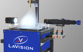
北京欧兰科技发展有限公司为您提供《空气击穿中阴影成像检测方案(激光产品)》,该方案主要用于其他中阴影成像检测,参考标准《暂无》,《空气击穿中阴影成像检测方案(激光产品)》用到的仪器有PL2250 闪光灯泵浦皮秒Nd:YAG激光器、Ekspla SFG 表面和频光谱分析系统、LaVision ParticleMaster-Shadow 粒径测量系统。
我要纠错
推荐专场
其它光谱仪
更多


相关方案
 咨询
咨询