

方案详情文
智能文字提取功能测试中
使用格哈特公司全自动凯氏定氮仪 VAPODEST维普得 检测玉米、冬油菜和冬小麦田中土壤总氮含量MDPIatmosphere 2 of 16Atmosphere 2023,14,372 用涡流协方差系统测量玉米、冬油菜和冬小麦田二氧化碳通量的时间动态Article Temporal Dynamics of CO2 Fluxes Measured with EddyCovariance System in Maize, Winter Oilseed Rape and WinterWheat Fields Robert Czubaszek *iDand Agnieszka Wysocka-Czubaszek Faculty of Civil Engineering and Environmental Sciences, Bialystok University of Technology, Wiejska 45A Str.,15-351 Bialystok,Poland * Correspondence: r.czubaszek@pb.edu.pl check forupdates Abstract: The full understanding of variation and temporal changes in carbon dioxide (CO2) fluxesin cropland may contribute to a reduction in CO2 emissions from agriculture. The aim of this studywas to determine the CO2 exchange intensity in the three most popular crops in Poland. The CO2fluxes in summer maize, winter oilseed rape and winter wheat fields were measured using theeddy covariance system. The seasonal dynamics of CO2 fluxes for all studied crops varied fromeach other due to individual dynamics in atmospheric CO2 assimilation of each species through thegrowing season. The weighted average values of CO2 fluxes calculated for the entire vegetationperiod were -22.22 umol CO2 m-2s-1, -14.27 umol CO2 m-2s-1 and -11.95 umol CO2 m-2s-1for maize, oilseed rape and wheat, respectively. All the studied agro-ecosystems were carbon sinksduring the growing season. The highest negative values of CO2 fluxes (-36.31 umol CO2 m-2s-1and -33.56 umol CO2 m-2s-l) were observed in the maize field due to the high production ofbiomass. However, the maize field was also the most significant carbon source due to slow growthof plants at the beginning of the growing season, and due to leaving the field fallow after harvestuntil the next sowing. In these two periods, the CO2 fluxes ranged from 0.59 umol CO2 m-2s-1to 3.72 umol CO2 m-2s-1. CO2 exchange over wheat and oilseed rape fields was less intense,but more even throughout the growing season. In the wheat field, the CO2 fluxes ranged from-1.70 umol CO2 m-2s-1 to -23.49 umol CO2 m-2s-l and in the oilseed rape field they rangedfrom -1.40 umol CO2 m-2 s-1 to -22.08 umol CO2 m-?s-1. In addition, the catch crop in theoilseed rape field contributed to the intensive absorption of CO2 after harvesting the main crop. Keywords: CO2 fluxes; eddy covariance; plant development stage; maize field; winter oilseed rapefield; winter wheat field; cropland Chong Shi, Nan Li and Xingjun Xie 1. Introduction Received: 30 December 2022 Revised: 7 February 2023 Accepted: 11 February 2023 Published: 14 February 2023 European Member States are committed to shift into a climate neutral economy by2050 [1]. European Climate Law sets the intermediate target of reducing greenhouse gas(GHG) emissions by at least 55% by 2030 [2]. The transition to a neutral-climate continentrequires the commitment and contribution of all sectors. In 2021, the EU Members emitted3,641,710.673 kt CO2 eq. [3]. The manufacturing and energy sectors were responsible forthe most emissions, followed by transportation and agriculture [4]. Copyright: @ 2023 by the authors.Licensee MDPI, Basel, Switzerland.This article is an open access articledistributed under the terms andconditions of the Creative CommonsAttribution (CC BY) license (https://creativecommons.org/licenses/by/4.0/) According to IPCC methodology [5], GHG emissions from agriculture include: entericfermentation (CH4), manure management (CH4,N2O),agricultural soils (CO2, CH4 N2O),field burning of agricultural residues (CH4, N2O), liming (CO2) and urea application(CO2). More than 80% of total agricultural GHG emissions are CH4 emissions from entericfermentation and N2O emissions from soils in Europe [6]. Both those gases have muchhigher 100-year global warming potential (GWP-100) than carbon dioxide (CO2),equalto 273, 27 and 29.8 for N2O, CH4-non fossil and CH4-fossil, respectively [7]. Therefore,despite a relatively small share in total GHG emissions equal to~13% [4], the agricultural sector has great potential to reduce its emissions [8] since this sector is responsible for 53%of CH4 emissions [9]. GHG emissions from agriculture are related to cultivation, varietyof crops, rearing livestock and related equipment and can be categorized in three tiers ofcarbon footprinting: (1) energy input through machinery, electricity, livestock managementand fossil fuels; (2) crop cultivation;(3) land use changes including conversion of naturalecosystems to agriculture and deforestation [10]. Poland is one of the main agricultural producers in the EU. In 2021, Poland harvested34.0 million tonnes of cereals (11.4% of EU total) and was the third country after France(66.9 million tonnes; 22.5% of EU total) and Germany (42.4 million tonnes; 14.3% of EUtotal). The harvested rape and turnip rape seeds were equal to 3 million tonnes in 2021 andcontributed 18% to the EU's total [11]. In Poland, cereal covers the highest crop area, followed by industrial crops and foddercrops. In cereal production, winter wheat is the main crop; in industrial crops, the oilseedrape has the highest share; and in fodder crops, maize dominates. Maize is an importantfodder in Polish agriculture which is based on cereals and dairy cow production. Wheatcovers ~30% of cereals area and contributes ~35% in cereal crops. Rape oilseed is the mainraw material for edible oil produced in Poland. Maize and oilseed rape are also the mainraw materials for biofuel production. Maize silage is one of the most important feedstocksfor biogas production while oilseed rape is used for biodiesel production [12]. The GHGemissions from raw material production for fuel purposes may decide if biofuel can beconsidered sustainable and socially acceptable. In Poland, the average GHG emissionsgenerated in the production of rapeseed for fuel equals to 24.28 g CO2 eq. MJ[13]. Maizecultivation generates 77.1 kg CO2 eq. tpM-1[14]. Carbon flux in both natural and cultivated ecosystems has seasonal variations closelyrelated to plant growth [15,16]. The carbon fluxes in cropland are related to human activitysuch as agronomic measures, the planting pattern or in some regions, the irrigation sys-tem [17]. In the vegetation period, or more precisely between sowing and harvest, cropsmay serve as a carbon sink [16,18]. In pea and maize cropping systems, the CO2 uptakeoffsets N2O and CH4 emissions [18]. The wheat, maize and wheat-maize cropping systemsalso behave as GHG sinks because of C sequestration [19]. Verma et al. [20] also reportedthat the rainfed maize-soybean rotation system is C neutral. If irrigation is used, the samerotation becomes a moderate C source, while continuously irrigated maize is nearly Cneutral or a slight C source. Peng et al. [21], however, reported that maize cropping systemsare a net carbon source if the carbon input with seeds and output at harvest are taken intoaccount. The comparison of wheat and maize revealed that wheat is a weak C sink, whilemaize is close to CO2 neutral to the atmosphere. However, when considering the totalCO2 loss in the fallow period, the full crop cultivation cycle of both crops were weak CO2sources [22]. The crop rotation is one of the most crucial factors affecting the C budget.Lehuger et al. [23] reported that wheat-maize-barley rotation was a net C source whileoilseed rape-wheat-barley rotation was a net C sink due to higher C sequestration and Creturn from crops. Results given by Wen et al. [24] revealed that oilseed rape crops behaveas C sinks and the sequestration potential rises with the growth stage in the followingorder: flowering stage, pod stage, bolting stage and seedling stage. The objective of thisstudy was to determine the CO2 exchange intensity in three different crops during thesame growing season and identify the crop which is characterized by the highest reductionin CO2 emission throughout the vegetation period. We hypothesize that: (1) there aredifferences in CO2 fluxes in three different crops (summer maize, winter oilseed rape andwinter wheat) and (2) the fluxes are influenced by crops and biomass growth. 2. Materials and Methods 2.1. Study Site Three adjacent fields located 19 km south of Bialystok, Poland (53°17'N, 23°11'E,147 m a.s.l.) were chosen to conduct the CO2 flux measurements. The study was conductedin similar microclimatic conditions on arable fields with most popular crops in Poland such 2.2. Experimental setup The CO2 fluxes (CO2 exchange between plant canopy, soils and atmosphere) withother microclimatic conditions (air temperature (Ta), air relative humidity (RH), solarradiation (Rg), net radiation (Rn), photosynthetic photon flux density (PPFD), soil heatfluxes (SHF), soil water content (SWC), soil temperature (Ts), plant cover and plant heightwere determined on monthly or two week bases in all three fields in 3 measurementcampaigns from spring 2016 to autumn 2016. The CO2 fluxes in wheat field were measuredon 8 test days: April 20, May 20, June 7, June 21, July 4, July 18, August 12, September 1.In oilseed rape field, the measurements were conducted on 10 test days: April 26, May11, May 24, June 9, June 24, July 5, July 18, August 12,September 1 and September 14. Inmaize field, 7 test days were performed: May 13, May 19, June 6, June 14, June 28, July25 and September 2. The dates of measurements were chosen so that no agrotechnicaltreatments were carried out at that time and, therefore, the emissions from fertilizers andfuel consumption were not taken into account in this study. Soil physicochemical parameters were determined from samples taken in May (maize)and June (oilseed rape and wheat). Plant cover was measured using the digital photographsin squares of 1 m2. We used a software program Corel PHOTO-PAINTTM (CorelDRAW@Graphics Suite, Alludo, Ottawa, Canada) to divide the images into different ground coverclasses based on the similarities among the pixels. The height of plants was measured withthe meter stick in the field. 2.3. Soil Sampling and Analysis 2.4. Eddy Covariance Measurements The fluxes in CO2 were measured with eddy covariance (EC) system which con-sisted of LI-7500A (LI-COR Biosciences, Lincoln, NE, USA) open-path analyser to measureCO2/H2O concentrations and sonic anemometer WindMaster (Gill Instruments Limited,Lymington, UK) to measure three-dimensional wind speed, wind direction and sonictemperature. Measurements were conducted with a frequency of 10 Hz. Due to the fact that this study aimed to directly compare variations in CO2 flux in different crops duringgrowing season, the EC system was moved among three studied crop fields (Figure 1).Each test day, EC system was installed in various parts of the currently studied crop field,depending on the wind direction, so that the results were obtained each time from thestudied crop field. In order to have sufficient fetch which represents studied crop field, allsensors were fixed 200 cm above the ground or canopy layer. In the maize field, a geodeticstand was used to reach the required height. The measurements were conducted between10:00 a.m. and 2:00 p.m. to minimize the diurnal variation in flux patterns since at this timeof the day the wind conditions were the most stable in terms of speed and direction. Earlierin the morning, the wind speed was too low, while in the afternoon, wind direction waschanging hampering the flux measurement from the studied field. The hourly interval waschosen based on the earlier observations of wind conditions. Nevertheless, the choice ofmeasurement protocol with relatively short measurement period resulted in the lack ofimportant information related to gas exchange. During all measurements, friction velocity(u*) was above 0.15 ms-. Figure 1. Location of eddy covariance tower (pink spots) on every test day on winter wheat, oilseedrape and maize fields. Data logger Xlite 9210 (Sutron, Sterling, VA, USA) was used for recording the datafrom EC sensors. In order to refine the final CO2 fluxes from the study fields, they werecalculated for periods of 5 min using the EddyPro5 software package. The followingcalculation procedures were applied: spectral corrections [30,31]; compensation for densityfluctuations [32]; sonic temperature correction for humidity [33]; time lag adjustment;coordinator rotation; block averaging; and statistical tests [34]. The footprint was estimatedaccording to Kljun et al. [35]. Daily fluxes were calcul1ated as extrapolation betweenmeasured values and weighted average for the vegetation period was calculated on thebasis of daily CO fluxes and days. During flux measurements, microclimate of the currently studied field was analysedwith the following set of sensors connected to the data logger: pyranometer sensor LI-200SL-50 (LI-COR, Lincoln, NE,USA), quantum sensor LI-190SL-50 (LI-COR, Lincoln, NE,USA), net radiometer NR Lite2, (Kipp&Zonen, Delft, The Netherlands), air temperature andrelative humidity probe HMP155, (Vaisala OYJ, Vantaa, Finland), three soil heat flux platesHFP01 (Hukseflux Thermal Sensors B.V., Delft, The Netherlands), three soil temperatureand water content sensors Hydra Probe II (Stevens Water Monitoring System Inc., Portland,OR, USA). Metrological data were recorded every 1 min. The sensors of soil temperature and water content were inserted vertically into soil surface and heat plates were installedat depth of 5 cm. 2.5. Statistical Analyses The significant differences in chemical properties amongst soils from all studied fieldswere assessed with one-way analysis of variance (ANOVA). Differences between meanswere determined using Tukey’s test. The homogeneity of variance and normality waschecked prior to ANOVA using the Brown-Forsythe and Shapiro-Wilk tests, respectively.When data failed the Shapiro-Wilk test, the F Welsh test was used for assessment of the signif-icance of differences amongst the chemical properties. The Kruskal-Wallis test was performedwhen data failed the Brown-Forsythe test, indicating the inhomogeneity of variance. Thesignificant differences amongst CO2 fluxes were also analysed with the Kruskal-Wallis test.Spearman correlation coefficients were calculated for CO fluxes and microclimatic variablesto point out the main factors that influenced values of CO2 fluxes. The level of acceptedstatistical significance was p<0.05. All the statistical analyses of data were performed usingSTATISTICA 13.3 software (TIBCO Software Inc., Palo Alto, CA,USA). 3. Results 3.1. Soil Properties In the maize and oilseed rape fields, the topsoil texture is loamy sand and in thewheat field, sandy loam dominates. The pH in all the soils indicated the slightly acidicconditions (Table 1). The SOC content was similar in the soil from the maize field andfrom the wheat field, even though these soils were characterized by different texture.The SOC concentration in the soil from oilseed rape was significantly (p<0.05) lower.Contradictory, total N content was significantly higher (p <0.05) in the soil from the wheatfield compared to soils from the maize and oilseed rape fields. These differences resulted ina significantly (p<0.05) higher C/N ratio in soil from the maize field. The plant-availablephosphorus content followed the pattern of total N; however, its concentration in the soilfrom wheat was twofold lower than its content in the two other studied soils. In the soilsfrom maize and oilseed rape, P20s concentration was remarkably high and in the soil fromwheat, it was average, according to the Egner-Riehm limit values [36]. The plant-availablepotassium concentration in all soils ranged from 17.3 ±8.5 mg 100 g- to 22.3±0.8 mg100 g-1. Since K2O concentration in the two soils from the oilseed rape and the wheat fieldswere characterized by very high variability, there was no statistically detected differencesamong ll studied soils. According to the Egner-Riehm limit values [36], the averagesoil from the maize field was characterized by remarkably high K2O content, the soil fromthe oilseed rape field had high K2O concentration, while in the soil from the wheat field,average K2O content was observed. Table 1. Soil properties (means ± standard deviations) from wheat, maize and oilseed rape fields. Crop Soil Texture Soil Fraction (mm) pH SOC N C/N P2O5 K2O 2-0.05 0.05-0.002 <0.002 H2O KCI Maize 79±1a 20±1a 1±1a 6.5±0.4a 5.6±0.4a 12.0±0.4a1.0±0.1a 11.6±0.4a 28.7±2.3a 22.3±0.8a Oilseed 74±4a 24±3a 2±1a 6.3±0.2a 5.4±0.5a 9.1±1.8b 0.9±0.2a 9.4±0.5b 29.7±10.4a 17.3±8.5a rape Wheat 66±3b 30±1b 4±2b 6.5±0.6a 5.6±0.9a 13.8±1.0a 1.5±0.2b 9.1±0.3b 12.5±4.3b 18.0±5.6a Soil texture-content of soil fractions (%), pH-reaction, SOC-soil organic carbon (g kg), N-total nitro-gen (g kg-), P20s-plant-available phosphorus (mg 100 g-), K2O-plant-available potassium (mg 100 g-).Lowercase letters—statistical differences at p <0.05. 3.2. Meteorological and Soil Conditions The meteorological conditions prevailing in the study area during the measurementswere relatively even (Table 2). Ta was ~20 °C for most of the study period, while RHwas ~50%. In most measurement days, PPFD exceeded the value of 1000 umol m-2s-1,fostering the process of photosynthesis. The maximum value of 1740.68 umol m-2s-1 wasreached during measurements over the oilseed rape field. Values lower than 1000 umol m-2s-1were observed only on three measurement days Table 2. Microclimatic conditions during measurements in the studied fields. Date Ta RH Rg Rn PPFD SWC Ts Wheat field April 20 9.64 49.69 552.79 313.70 1133.70 0.17 14.83 May 20 17.49 50.00 683.15 443.54 1369.88 0.20 22.69 lune 7 16.04 39.74 830.96 547.33 1666.39 0.17 24.07 June 21 18.96 74.83 587.12 425.87 1221.42 0.17 22.81 July 4 19.48 53.25 567.84 376.98 1162.47 0.20 21.63 July 18 20.36 55.84 559.99 433.82 1220.34 0.23 23.58 August 12 17.61 47.44 651.69 408.85 1308.96 0.26 16.36 September 1 20.51 54.32 529.41 267.87 1076.29 0.10 25.21 Oilseed rape field April 26 7.51 58.36 459.62 246.06 931.03 0.07 11.60 May 11 21.07 48.60 597.37 358.03 1129.51 0.05 20.98 May 24 22.59 38.06 846.81 528.68 1740.68 0.06 20.66 June 9 15.92 49.67 766.30 496.95 1564.39 0.07 20.52 June 24 27.76 53.25 777.71 555.45 1631.78 0.05 25.96 July 05 21.50 45.58 726.03 511.83 1284.06 0.08 24.48 July 18 18.65 61.79 399.62 281.93 768.36 0.18 19.85 August 12 18.21 43.79 531.09 290.68 1055.89 0.15 23.39 September 1 21.65 52.65 571.11 330.57 1212.29 0.05 27.98 September 14 19.86 50.59 632.60 327.22 1355.50 0.03 26.46 Maize field May 13 20.64 49.87 535.68 304.11 1126.53 0.09 26.29 May 19 15.40 29.47 398.19 214.14 808.27 0.13 20.40 June 3 22.65 43.70 799.48 498.77 1629.50 0.14 30.03 Tune 14 20.57 44.93 568.70 327.36 1164.00 0.04 25.92 June 28 20.67 55.36 524.84 330.34 1076.65 0.02 28.83 July 25 26.50 60.25 779.95 529.63 1554.20 0.04 35.79 September 2 21.79 55.43 662.98 328.18 1338.19 0.02 27.07 Ta-air temperature (C), RH-air relative humidity (%), Rg-solar radiation (W m-2), Rn-net radiation(W m-2), PPFD-photosynthetic photon flux density (umol m-2s-1), SWC-soil water content (m’m-3), Ts-soiltemperature (°C). In all studied fields, Ts was similar. The only difference among the studied soils wasobserved for the SWC which was higher in the wheat field, characterized by slightly finermaterial of sandy loam, compared to loamy sand in the maize and oilseed rape fields. 3.3. Vegetation Development In the wheat field, the measurements started on April 20 in the wheat tillering phase,when plants with a height of ~10 cm covered~10% of the field (Figure 2). In the tilleringstage, the wheat growth was relatively slow, since within a month, plants reached 35 cmand covered about 40% of the field and entered the stem elongation stage. In the next twoweeks, the wheat growth rate accelerated and plants with a height of 80 cm covered ~80%of the field. In the flowering stage, both the height and the degree of coverage of the fieldby vegetation changed only slightly. Wheat reached the development of fruit stage at the beginning of August and entered the senescence stage in the second half of July. The heightof the plants and cover was stable in this period until the harvest on August 20. Figure 2. Vegetation development in the wheat field. The field measurement in the oilseed rape started on April 26 when plants werealready ~40 cm high and covered ~25% of the field (Figure 3). In the next two weeks, theplants grew to 90 cm in height and almost completely covered the field. At the end ofthis period, plants started the flowering stage which lasted altogether four weeks. In theflowering stage, the crop is in full flower which means that 50% of flowers on the mainraceme are open. This is accompanied by yellow colour in the crop field. On June 9, plantswere in the fruit development stage, when elongated green pods develop from pollinatedoilseed rape flowers. The next measurement on June 24 was performed on the plants inIe以the seeds ripening stage, in which pods at first are soft and green and in next 10 days theyturn brown. At the senescence stage, seeds became hard and black and the plants wereharvested at the end of July. Oilseed rape was followed by charlock sown for green manure.Initially, charlock covered a small area of the field, but after reaching a height of ~25 cm,almost the entire field was covered with a green cover. Figure 3. Vegetation development in the oilseed rape field. In the maize field, the first measurement was conducted on May 13, just after theemergence stage. In the first leaf collar stage, plants were 6 cm high and covered about 1%of the area (Figure 4). The maize was sown at an average of 12 plants per m2. A week later,the plants in the second leaf collar stage were ~10 cm high and covered 3% of the field. Inthe next two weeks, the plants grew faster, reaching a height of 40 cm and covering 30% ofthe field, entering the stem elongation stage. In this stage, in the next 10 days, the maizegrew to 80 cm and covered about 50% of the area. During the following two weeks, stillin stem elongation stage, plants reached a height of 140 cm and covered ~70% of the field.From that moment, the plant cover increased very slowly, even though the maize was stillgrowing. On the next measurement day (July 25), the plants reached 220 cm and were inthe flowering stage. For the next month, the plant cover was rather stable. The maize washarvested on September 7 at the end of the fruit development stage and ploughing tookplace the next day. The field was left fallow for winter. Figure 4. Vegetation development in the maize field. 3.4. CO2 Fluxes The seasonal dynamics of CO2 fluxes in winter wheat and oilseed rape were similar butdiffered significantly (p<0.05) from maize due to the individual dynamics in atmosphericCO2 assimilation of each species through the growing season (Figure 5). The CO2 absorptioncapacity is related to the vegetation development stage since changes in biomass and thelevel of chlorophyll in plants affects the photosynthesis process. Figure 5. The CO2 fluxes in wheat, oilseed rape and maize fields. During the tillering stage of wheat growth, despite the slight enlargement in biomass,the CO2 flux increased to over -20 umol CO2 m-2s-1 and remained on this level till theend of June. Thus, during the fast-growth stage of stem elongation, the photosynthesisexceeded the respiration. In the next stages, from flowering to senescence, the significantdrop in the CO2 absorption from the atmosphere was observed related to the decrease inchlorophyll levels indicated by colour change in the plants (Figure S1). Nevertheless, theCO2 flux was negative, indicating that the respiration was lower than photosynthesis forall the growing season. Similar seasonal dynamics in CO fluxes were observed for oilseed rape; however,from April to mid-May, the CO2 flux slightly exceeded the values measured for wheat.The negative values indicate that photosynthesis in the inflorescence emergence stagewas higher than respiration. The constant drop in CO2 fluxes was observed from May 11,indicating that in the next growth stages, beginning from the flowering stage through tothe fruit development and ripening stages, carbon capacity of the oilseed rape field wasgetting weaker (Figure S2). The lowest value of -1.7 umol CO2 m-2s-1 was reached onJuly 18 in the senescence stage. The increase in CO2 absorption in August was related tothe growth of charlock as a cover crop in the field after the oilseed rape was harvested atthe end of July. Contrary to the wheat and oilseed rape, CO2 assimilation by the maize field was themost intensive in the second half of the vegetation period, when plants were finishingthe stem elongation stage (Figure S3). In the first month of the study, when the plantcover was less than 30% of the field and the plants were ~30 cm high (Figure S3),CO2absorption reached a value similar to that of the wheat and oilseed rape fields. A furtherincrease in maize biomass in the next two weeks resulted in the CO, flux of more than-35 umol CO2 m-2s-1, indicating rising carbon absorption of the maize field during thistime. The CO flux remained at a similar level for the next two weeks, indicating thatthe photosynthesis was much stronger than respiration. During the next 6 weeks, dueto a gradual decrease in the intensity of photosynthesis, the CO2 flux dropped to about-20 umol CO2 m-2s-1. The weighted average values of CO2 fluxes calculated for the entire vegetation periodwere -22.22 umol CO2 m-2s-1,-14.27 umol CO2m-2s-1 and -11.95 umol CO2 m-2s-1for maize, oilseed rape and wheat, respectively. Conversion of these values into theamount of assimilated carbon revealed the following results: -160 g CO2-C ha-1 min-1,-102 g CO2-C ha-1 min-1 and -86 g CO2-C ha-1 min-1 for maize, oilseed rape andwheat, respectively. The field cultivation after harvest affected the annual CO2 fluxes. The wheat andoilseed rape were harvested at the end of August while maize was mown in late August andearly September. Leaving the maize field after harvest uncovered with any crop (Figure S4)resulted in positive values of CO2 flux, indicating the loss of CO2 assimilation and thestart of CO2 emissions. In the wheat field, after harvest, the CO2 fluxes were still negative,indicating the higher CO2 absorption over respiration. Indeed, weeds covered the soilbelow the wheat canopy in the senescence stage and after the crop harvest; they continuedto support photosynthesis. The oilseed rape harvest was followed by charlock as a covercrop. The rapid growth of charlock resulted in the development of almost complete plantcover in the field and negative values of CO2 fluxes, indicating growing carbon absorptioncapacity of the oilseed rape field after harvest. In the wheat field, CO2 fluxes were significantly (p<0.05) correlated with PPFD, Rgand Rn as well as with Ts (Table 3). In the case of oilseed rape, correlations with all analysedparameters were significant (p<0.05), with CO2 fluxes positively correlated with SWC andTs. In the maize field, the relationship between CO2 fluxes was significant (p<0.05) withTa, RH, Rn, SWC and Ts, but was only positive for SWC. Table 3. Correlation between CO fluxes and microclimatic conditions in the studied fields. CO2 Flux Ta RH Rg Rn PPFD SWC Ts Wheat field CO2 flux 1 -0.03 -0.11 -0.46 -0.47 -0.44 -0.01 -0.47 Ta 1 0.49 0.11 0.27 0.14 0.35 0.53 RH 1 -0.24 -0.14 -0.22 -0.13 0.06 Rg 1 0.97 0.99 0.18 0.30 0.98 PPFD 0.17 Rn 1 0.21 0.41 1 0.32 SWC 1 0.32 Ts 1 Oilseed rape field CO2 flux 1 -0.14 0.21 -0.33 -0.26 -0.38 0.62 0.15 Ta 1 -0.46 0.45 0.48 0.39 -0.37 0.56 RH 1 -0.58 -0.52 -0.51 0.05 -0.31 Rg 1 0.96 0.91 -0.12 0.29 Rn 1 0.87 -0.04 0.28 PPFD 1 一0.21 0.26 SWC 1 -0.37 Ts 1 Maize field CO2 flux -0.20 -0.14 -0.07 -0.21 -0.04 0.44 -0.38 Ta -0.05 0.56 0.57 0.58 -0.14 0.86 RH -0.02 -0.06 -0.05 -0.50 1 1 1 0.02 Rg 1 0.92 0.96 0.16 0.54 Rn 1 0.86 0.17 0.59 PPFD 1 0.14 0.56 SWC 1 -0.17 Ts 1 Ta-air temperature (C), RH-air relative humidity (%), Rg-solar radiation (W m-2), Rn-net radiation(W m-2), PPFD-photosynthetic photon flux density (umol m-2s-1), SWC-soil water content (m’m-3), Ts-soiltemperature (C). Bold values show significant correlations (p<0.05). 4. Discussion 4.1. Soil Properties and Plant Growth Winter wheat is highly resistant to low temperatures during the early stages of plantdevelopment and near freezing temperatures in this growth phase are required for vernal-ization [46]. Wheat is grown as a rainfed crop; however, this plant requires relatively highsoil moisture, especially for germination and several growth stages in autumn and spring.The adequate amount of stored water is particularly important due to a less developedroot system. Excessive rainfalls, especially in the period from earing to the end of ripeningare also unfavourable [47,48]. Growth is then prolonged, and plants can be easily affectedby diseases [47]. Wheat has the highest soil requirements of all cereals mainly due to aless developed root system and, therefore, a lower ability to take up nutrients. Wheatgrows best on well-drained, well-structured soils with high water capacity [48]. A soil pHbetween 6.0 and 7.0 is optimal for micronutrient availability and wheat growth. The mostlimiting factor is the N content in soil. Its deficiency leads to lower crops while its excessincreases plant susceptibility to diseases, lodging and spring freeze damage [49]. In thisstudy, the soil from the wheat field was characterized by a pH of 6.5 (Table 1), which isin the optimum range for wheat growth. Sandy loams with a high SOC and N contentand a remarkably high content of plant-available P and K (Table 1) were favourable forwheat cultivation. A higher content of clay and silt compared to loamy sands from themaize and oilseed rape fields might increase the water capacity and, thus, create goodwater conditions for wheat growth reflected by a higher SWC on all test days (Table 2). Oilseed rape grows best in a temperate climate and during its lifecycle it can beexposed to extreme temperatures; however, in the flowering stage it is very susceptible toeven short periods of drought. Water stress decreases the leaf area index (LAI), nitrogennutrition index and leaf chlorophyll [50]. Oilseed rape has remarkably high nutritional andwater requirements. The crop grows best on deep, medium-textured, well-drained, humusand calcium-rich soils [51] with an optimum pH at 5.7-7.0. Sandy, poor, acidic and drysoils, or heavy, waterlogged soils are unsuitable for oilseed rape cultivation [51]. In thisstudy, the soil from the oilseed rape field was characterized by pH 6.3, which was in theoptimum range. The content of plant-available P and K was remarkably high and despitethe low SOC content, the C/N ratio was narrow, which indicates a rapid rate of organicmatter transformation. 4.2. CO2 Fluxes 4.2.1. CO2 Fluxes from Agro-Ecosystems Various ecosystems, including agricultural land, can act both as a sink and as a sourceof carbon [52], and even slight changes during growing season can result in annual changesin CO flux. The net ecosystem exchange of CO2 refers·上IL to the difference between thecarbon fixation in photosynthesis and its release because of ecosystem respiration [53].The net vertical CO2 flux has a specific value and return. Negative net flux indicatesthe CO2 transport downwards to the active surface, i.e., the predominance of absorptionprocesses over emission. In turn, a positive net flux indicates the upward transport fromthe active surface to the atmosphere, i.e., the predominance of emissions over absorption.Soil cultivation is another source of significant GHG emissions including emissions fromthe use of mineral fertilizers and fuel and emissions from soil, which are the main sourcesof CO2 and N2O. However, proper agronomic practices often supply the soil with organicmatter and reduce the intensity of its decomposition and, thus, increase the carbon stockin the soil [54]. In this study, the CO2 fluxes (CO2 exchange between plant canopy, soilsand atmosphere) were measured on days in which the agrotechnical practices were notperformed, therefore the CO2 emissions from them were not included. This allowed usto focus only on CO2 emissions and the absorption of the studied agro-ecosystems andrecognize them as a C sink during the growing period. 4.2.2. Effect of Plant Development Stages on CO2 Fluxes CO2 emissions from agricultural land can be offset through the binding of this com-pound with the growing vegetation through photosynthesis. However, the efficiency ofthis process depends to a considerable extent on the rate of vegetation development aswell as on the land use. According to the research of Xu and Baldocchi [55], seasonaltrends in carbon fluxes in agro-ecosystems follow closely the change in the development ofplant cover, which is the result of the phenological phases of plants. In the studies of Janset al. [56], maximum daily CO2 fluxes in a corn field were associated with a peak growthperiod. A strong relationship between CO2 fluxes and the size of the plant cover expressedby the LAI was also shown by Wang et al. [57]. Liu et al. [53] also reported a rapid increasein CO2 flux in the fields covered by winter oilseed rape when the plants turned green, withits maximum at the jointing-booting and heading-filling stages, and a gradual decrease atthe milk ripening-maturity stage. These changes resulted from lower LAI, chlorophyll andenzyme content during the early growth stage of wheat, which determined a relatively lowphotosynthetic efficiency of plants. LAI, chlorophyll content and enzymatic activity reachedtheir maximum with wheat growing stages; thus, the plants were capable of relatively highphotosynthesis during the flowering phase. In the later part of the growing season, bothenzyme activity and chlorophyll content decreased due to the aging of the leaves, whichresulted in a decrease in the intensity of photosynthesis In this study, both wheat and oilseed rape relatively quickly fully covered the field,which resulted in the whole area of the field participating in the photosynthesis process. Atthe same time, sparsely planted maize left a significant area of the field uncovered withleaves. In mid-June, CO2 assimilation by maize rapidly increased, while in the case of thewheat and oilseed rape, the CO absorption decreased as a result of entering the stage offlowering and developing of fruits which in both plants was manifested by the loss of thechlorophyll responsible for photosynthesis. In the same period, maize growing graduallycovered the entire field, which resulted in the maximum intensity of CO2 assimilationwhich started at the end of June in the stem elongation stage and lasted on a stable levelthrough the flowering stage until the development of fruit stage at the end of August. 4.2.3. CO2 Flux Values in Winter Wheat, Oilseed Rape and Maize Fields Liu et al. [53] reported CO flux values in winter wheat field ranging from -1738 mgCO2 m-2 h-1 to -541 mg CO2 m-2h-1 in two studied growing seasons. In our study, thisrange was much wider from -3721 mg CO2 m-2h-1 to -537 mg CO2 m-2h-1. Despitethis difference, the relationships between CO2 assimilation and vegetation developmentfound in the analysed agro-ecosystems were similar. Eshonkulov [58] reported -198 gCO2-C ha-1 min-1 for a wheat field. This value is higher than that observed in thisstudy (-169 g CO2-C ha-1 min-1). In this study, in the oilseed rape field, the maximumvalue of the CO2 flux was observed on May 11 when it reached the value of -158 gCO2-C ha-l min-1. This value is slightly higher than that reported by Eshonkulov [58],who also observed a value of -142 g CO2-C ha-1 min-1 for an oilseed rape field in May.In the maize field, several months shift in the maximum CO2 flux compared to the wheatfield and the oilseed rape fieldwhich was observed in this study, is in a good agreementwith the results revealed by Eshonkulov [58] who reported a maximum flux in August equalto -211 g CO2-C ha-1 min-1, which is a much lower value compared to the result of thisstudy (-262 g CO2-C ha-min-1). The fluxes observed in the maize field in this study arehigher than the values presented by Zhang et al. [59], who studied the daily distribution ofCO2 exchange over various ecosystems and reported a maximum value for maize equal to-193 g CO2-C ha-1 min-1. 4.2.4. Effect of Microclimatic Variables on CO2 Fluxes CO2 exchange between terrestrial ecosystems and the atmosphere depends to a largeextent on environmental variables [60]. Liu et al. [53] found that CO2 fluxes are significantlycorrelated with PPFD, Ta, Ts, RH and SWC. Solar radiation is crucial for the photosynthesisprocess, therefore, among the factors listed above, PPFD is particularly important for thedaily course of CO2 flux. In this study, the value of this parameter remained at a highlevel, which was conducive to gas exchange. This process was also supported by otherparameters measured in this study, i.e., solar radiation (Rg) and net radiation (Rn). The lackof a significant relationship between CO2 fluxes and PPFD in the maize field was relatedto the low impact of this radiation on the absorption of CO2 by poorly developed plantsthat covered a small area of the field. An equally positive effect on the process studied inthis work was the relatively high Ta and Ts, which are the predominant limiting factors forthe growth of plants and activity of the microbial community [57]. The SWC found in thisstudy was conducive to CO2 fluxes in all the studied fields. According to the research ofWang et al. [57], SWC higher than 0.25 m’m-3 may reduce gas exchange. This is becausehigher SWC reduces the water absorption rate of the root system leading to a decrease inthe photosynthesis rate. A significant negative linear relationship between SWC and CO2flux during the post-milk ripening period in winter wheat fields was demonstrated by Liuet al. [53]. The positive correlation of CO2 fluxes and SWC in oilseed rape and maize fieldsfound in this study is the result of low water content in the soil, which in such amountsfavours the development of plants, while not inhibiting the gas exchange process. 5. Conclusions In this study, the CO2 fluxes in summer maize, winter oilseed rape and winter wheatfields were measured using the eddy covariance system. The measurements were con-ducted from the early stage of plant development to the post-harvest period. This studyrevealed a large difference between maize and two other studied crops in terms of CO2exchange between the land surface and the atmosphere. Even though all the studied agro-ecosystems were carbon sinks, the intensity of carbon assimilation varied in individualfields during the study period. The highest negative values of CO fluxes, indicating strongabsorption of this gas in the photosynthesis process, were observed in the maize field dueto the high production of maize biomass. However, the maize field was a carbon sourcefor the greater part of the year due to slow growth of the plants at the beginning of thegrowing season, and due to leaving the field fallow after harvest until the next sowing.CO2 exchange in wheat and oilseed rape fields was less intense, but more even throughoutthe growing season. In addition, the catch crop in the oilseed rape field contributed to theintensive absorption of CO2 after harvesting the main crop. The differences in CO fluxesbetween fields resulted from the plants' physiology and agrotechnical treatments; but, dueto these features, the total amounts of carbon absorbed by the analysed crops are more eventhan the maximum CO2 fluxes would indicate. Supplementary Materials: The following are available online at https://www.mdpi.com/article/10.3390/atmos14020372/s1. Figure S1. The development stages of wheat on: 20 April 2016 (a), 20May 2016 (b),21 June 2016 (c), 18 July 2016 (d); Figure S2. The development stages of oilseed rape on:26 April 2016 (a), 11 May 2016 (b), 9 June 2016 (c), 5 July 2016 (d); Figure S3. The development stagesof maize on: 19 May 2016 (a), 14 June 2016 (b), 28 June 2016 (c), 2 September 2016 (d); Figure S4. Thesurface of the studied fields after harvest: a-wheat field,b-oilseed rape field, c—maize field. Author Contributions: Conceptualization, R.C.; methodology, R.C.; validation, R.C.; formal analysis,R.C. and A.W.-C.; investigation, R.C.; writing-original draft preparation, R.C.; writing-review andediting, A.W.-C.; visualization, R.C. and A.W.-C. All authors have read and agreed to the publishedversion of the manuscript. Funding: The research was carried out as part of project No. WZ/WB-IIS/1/2020 at the BialystokUniversity of Technology and financed from the research subsidy provided by the Minister ofEducation and Science. Institutional Review Board Statement: Not applicable Informed Consent Statement: Not applicable. Data Availability Statement: Not applicable. Conflicts of Interest: The authors declare no conflict of interest. The funders had no role in the designof the study; in the collection, analyses, or interpretation of data; in the writing of the manuscript; orin the decision to publish the results. References 1. European Commission. The European Green Deal. Communication from the Commission to the European Parliament, the EuropeanCouncil, the Council, the European Economic and Social Committee and the Committee of the Regions; COM (2019) 640 Final; EuropeanCommission: Brussels, Belgium, 2019. 2. Regulation (EU) 2021/1119 of the European Parliament and of the Council of 30 June 2021 Establishing the Framework forAchieving Climate Neutrality and Amending Regulations (EC) No 401/2009 and (EU) 2018/1999 ('European Climate Law'). Off.J. Eur. Union 2021, L 241,1-17. 3. European Environment Agency. GHG_proxy_2021. Available online: https://www.eea.europa.eu/data-and-maps/data/approximated-estimates-for-greenhouse-gas-emissions-5/2017-ghg-proxies/ghg_proxy_2017 (accessed on 29 November 2022). 4 Eurostat. File:Quarterly GHG Figures for Q2 2022 with GDP Ver2.Xlsx. Available online: https://ec.europa.eu/eurostat/statistics-explained /index.php?title=File:Quarterly_GHG_Figures_for_Q2_2022_with_GDP_ver2.xlsx (accessed on 29 November 2022). 5. Buendia, E.C.; Tanabe, K.; Kranjc, A.;Jamsranjav, B.; Fukuda, M.;Ngarize, S.;Osako, A.; Pyrozhenko, Y.; Shermanau,P; Federici, S.2019 Refinement to the 2006 IPCC Guidelines for National Greenhouse Gas Inventories, 1st ed.; IPCC: Geneva, Switzerland, 2019. 6. European Environment Agency. National Emissions Reported to the UNFCCC and to the EU Greenhouse Gas Monitoring Mechanism. Available online: https://www.eea.europa.eu/ims/greenhouse-gas-emissions-from-agriculture (accessed on 30November 2022). 7. IPCC. Climate Change 2021: The Physical Science Basis, 1st ed.; Contribution of Working Group I to the Sixth Assessment Report ofthe Intergovernmental Panel on Climate Change; Cambridge University Press: Cambridge, UK;New York, NY, USA, 2021. 8. Mielcarek-Bochenska, P.; Rzeznik, W. Greenhouse Gas Emissions from Agriculture in EU Countries-State and Perspectives.Atmosphere 2021,12,1396. [CrossRef] 9 van der Veen, R.; de Vries, M.; van de Pol, J.; van Santen, W.; Sinke, P.; de Vries,J.; Kampman, B.; Bergsma, G. Methane ReductionPotential in the EU between 2020 and 2030, 1st ed.; CE Delft: Delft, The Netherlands, 2022. 10. Jaiswal, B.; Agrawal, M. Carbon Footprints of Agriculture Sector. In Carbon Footprints; Muthu, S.S., Ed.; Environmental Footprintsand Eco-design of Products and Processes; Springer: Singapore, 2020; pp. 81-99. ISBN 9789811379154. 11. Eurostat. Agricultural Production-Crops. Available online: https://ec.europa.eu/eurostat/statistics-explained/index.php?title=Agricultural_production_-_crops (accessed on 5 December 2022). 12. Statistics Poland. Production of Agricultural and Horticultural Crops. Available online: https://stat.gov.pl/obszary-tematyczne/rolnictwo-lesnictwo/uprawy-rolne-i-ogrodnicze/produkcja-upraw-rolnych-i-ogrodniczych-w-2021-roku,9,20.html (accessedon 3 December 2022). 13. Borzecka-Walker, M.; Faber, A.; Jarosz, Z.; Syp, A.; Pudelko, R. Greenhouse Gas Emissions from Rape Seed Cultivation for FAMEProduction in Poland. J. Food Agric. Environ. 2013,11,1064-1068. 14. Wisniewski, P.; Kistowski, M. Greenhouse Gas Emissions from Cultivation of Plants Used for Biofuel Production in Poland.Atmosphere 2020, 11, 394.[CrossRef] 15. Li, H.; Zhang, F; Li, Y.; Wang, J; Zhang, L.; Zhao,L.; Cao, G.; Zhao, X.; Du, M. Seasonal and Inter-Annual Variations in CO2Fluxes over 10 Years in an Alpine Shrubland on the Qinghai-Tibetan Plateau, China. Agric. For. Meteorol. 2016,228-229,95-103.[CrossRef 16. Schmidt, M.;Reichenau, T.G.; Fiener, P.; Schneider, K. The Carbon Budget of a Winter Wheat Field: An Eddy Covariance Analysisof Seasonal and Inter-Annual Variability. Agric. For. Meteorol. 2012,165,114-126.[CrossRef] 17. Guo,H.; Li, S.; Wong, F.-L.; Qin, S.; Wang, Y.; Yang, D.; Lam, H.-M. Drivers of Carbon Flux in Drip Irrigation Maize Fields inNorthwest China. Carbon Balance Manag. 2021,16,12. [CrossRef] [PubMed] 18. Maier, R.; Hortnagl, L.; Buchmann, N. Greenhouse Gas Fluxes (CO2,N2O and CH4) of Pea and Maize during Two CroppingSeasons: Drivers, Budgets, and Emission Factors for Nitrous Oxide. Sci. Total Environ. 2022,849,157541.[CrossRef] 19. Tao,F.; Li, Y.; Chen, Y.; Yin, L.; Zhang, S. Daily, Seasonal and Inter-Annual Variations in CO2 Fluxes and Carbon Budget in aWinter-Wheat and Summer-Maize Rotation System in the North China Plain. Agric. For. Meteorol. 2022,324,109098. [CrossRef] 20. Verma, S.B.; Dobermann, A.; Cassman, K.G.; Walters, D.T.; Knops, J.M.; Arkebauer, T.J.; Suyker, A.E.; Burba, G.G.; Amos, B.;Yang, H.; et al. Annual Carbon Dioxide Exchange in Irrigated and Rainfed Maize-Based Agroecosystems. Agric. For. Meteorol.2005,131,77-96. [CrossRef] 21. Peng, X.; Ma, J.; Cai, H.; Wang, Y. Carbon Balance and Controlling Factors in a Summer Maize Agroecosystem in the GuanzhongPlain, China. J. Sci. Food Agric. 2023, 103,1761-1774. [CrossRef] [PubMed] 22. Zhang, Q.; Lei, H.; Yang, D.; Xiong, L.; Liu, P;Fang, B. Decadal Variation in CO2 Fluxes and Its Budget in a Wheat and MaizeRotation Cropland over the North China Plain. Biogeosciences 2020, 17, 2245-2262. [CrossRef] 25. Richling, A.; Solon, J; Macias, A.; Balon, J.; Borzyszkowski, J.; Kistowski, M. Regional Physical Geography of Poland, 1st ed.; BoguckiWyd. Naukowe: Poznan, Poland, 2021. (In Polish) 26. Gorniak, A. Climate of the Podlaskie Voivodeship in the Time of Global Warming, 1st ed.; Wydawnictwo Uniwersytetu w Bialymstoku:Bialystok, Poland, 2021. (In Polish) 27. IUSS Working Group WRB World Reference Base for Soil Resources 2014. Update 2015 International Soil Classification System forNaming Soils and Creating Legends for Soil Maps; FAO: Tome, Italy, 2015. PN-R-04032:1998; Soil Sample Collecting and An8alysis of Soil Texture. Polski Komitet Normalizacyjny: Warsaw, Poland, 1998. (In Polish) Ostrowska, A.; Gawlinski, S.; Szczubiatka, Z. Methods of Analysis and Evaluation of Soil and Plant Properties. Catalog, 1st ed.; InstytutOchrony Srodowiska: Warsaw, Poland, 1991. (In Polish) 30. Moncrieff, J.; Clement, R.; Finnigan, J.; Meyers, T. Averaging, Detrending, and Filtering of Eddy Covariance Time Series. InHandbook of Micrometeorology: A Guide for Surface Flux Measurement and Analysis; Atmospheric and Oceanographic Sciences Library; Lee, X., Massman, W., Law, B., Eds.; Springer: Dordrecht, The Netherlands, 2005; pp. 7-31. ISBN 978-1-4020-2265-4. 31. Moncrieff, J.B.; Masheder, J.M.; de Bruin, H.; Elbers,J;Friborg, T.; Heusinkveld, B.; Kabat, P.; Scott, S.; Soegaard,S.; Verhoef, A. A System to Measure Surface Flux Momentum, Sensible Heat, Water Vapor and Carbon Dioxide. J. Hydrol. 1997,188-189,589-611.[CrossRef] 32. Webb, E.K.; Pearman, G.I.; Leuning, R. Correction of Flux Measurements for Density Effects Due to Heat and Water VapourTransfer. Quat. J. R. Met. Soc. 1980,106,85-100. [CrossRef] 33. Van Dijk, A.; Moene, A.F; Debruin, H.A.R. The Principles of Surface Flux Physics: Theory, Practice and Description of the ECPACK Library;Internal Report 2004/1; Meteorology and Air Quality Group, Wageningen University: Wageningen, The Netherlands, 2004 34. Vickers, D.; Mahrt, L. Quality Control and Flux Sampling Problems for Tower and Aircraft Data. J. Atmos. Oceanic Technol.1997,14,512-526.[CrossRef] 35. Kljun, N.; Calanca,P.; Rotach, M.W.; Schmid, H.P. A Simple Parameterisation for Flux Footprint Predictions. Bound.-Layer Meteorol.2004, 112,503-523. [CrossRef] 36. Egner, H.; Riehm, H.; Domingo, W.R. Studies on Chemical Soil Analysis as a Basis for Assessing the Nutrient Status ofSoils. ⅡI. Chemical Extraction Methods for Phosphorus and Potassium Determination. Kungliga Lantbrukshogskolans Annaler1960,26,199-215. (In German) du Plessis, J. Maize Production, 1st ed.; Department of Agriculture, Republic of South A38frica: Pretoria, South Africa, 2003. Rutkowski, J. Technology of Maize Cultivation-From Sowing to Harvesting, 1st ed.; Warminsko-Mazurski Osrodek DoradztwaRolniczego: Olsztyn,Poland,2018. (In Polish) 39. Kaniuczak, Z.; Pruszynski, S. Methodology of Integrated Maize Production, 3rd ed.; Glowny Inspektorat Ochrony Roslin i Nasien-nictwa: Warsaw, Poland, 2020. (In Polish) 40. Cofas, E. The Dynamics of Maize Production in the Climate Factors Variability Conditions. In Proceedings of the AgrarianEconomy and Rural Development-Realities and Perspectives for Romania, 9th Edition of the International Symposium, Bucharest,Bucharest, 20-21 November 2018; The Research Institute for Agricultural Economy and Rural Development (ICEADR): Bucharest,Bucharest, 2018; pp. 239-245. 43. Pettigrew, W.T. Potassium Influences on Yield and Quality Production for Maize, Wheat, Soybean and Cotton. Physiol. Plant.2008,133,670-681. [CrossRef] [PubMed] 44. Madar, R.; Singh, Y.V.; Meena, M.C.; Das, T.K.; Gaind, S.; Verma, R.K. Potassium and Residue Management Options to Enhance Productivity and Soil Quality in Zero Till Maize-Wheat Rotation. Clean-Soil Air Water 2020, 48, 1900316. [CrossRef]45. Niu, J.;Zhang, W.; Chen, X.; Li, C.;Zhang,F; Jiang, L.; Liu, Z.; Xiao, K.; Assaraf, M.; Imas, P. Potassium Fertilization on Maize under Different Production Practices in the North China Plain. Agron. J. 2011,103,822-829. [CrossRef] 47. Horoszkiewicz-Janka, J.; Korbas, M.; Mrowczynski, M. Methodology of Integrated Protection of Winter and Spring Wheat for Producers,1st ed.; Instytut Ochrony Roslin Panstwowy Instytut Badawczy: Poznan, Poland, 2013. (In Polish) 48. Tomicka, I.; Bujnowska, Z. Crop Production, 2nd ed.; Panstwowe Wydawnictwa Rolnicze i Lesne: Warsaw, Poland, 1995; Volume 2.(In Polish) 49. Nleya, T. Chapter 4: Winter Wheat Planting Guide. Available online: https://extension.sdstate.edu/igrow-wheat-best-management-practices-wheat-production (accessed on 28 December 2022). 50. Zajac, T.; Klimek-Kopyra, A.; Oleksy, A.; Lorenc-Kozik, A.; Ratajczak, K. Analysis of Yield and Plant Traits of Oilseed Rape (BrassicaNapus L.) Cultivated in Temperate Region in Light of the Possibilities of Sowing in Arid Areas. Acta Agrobot. 2016,69,1-13. [CrossRef] 51. Pospisil, M.; Brěic, M.; Husnjak, S. Suitability of Soil and Climate for Oilseed Rape Production in the Republic of Croatia. Agric.Conspec. Sci. 2011,76,35-39. 52. Ray, R.L.; Griffin, R.W.; Fares, A.; Elhassan, A.; Awal, R.; Woldesenbet, S.; Risch, E. Soil CO2 Emission in Response to OrganicAmendments, Temperature, and Rainfall. Sci. Rep. 2020,10,5849.[CrossRef] 53. Liu, C.; Wu, Z.; Hu,Z.; Yin, N.;Islam, A.R.M.T.; Wei, Z. Characteristics and Influencing Factors of Carbon Fluxes in Winter WheatFields under Elevated CO2 Concentration. Environ. Pollut. 2022, 307,119480. [CrossRef] [PubMed] 54. Paustian, K.; Six, J; Elliott, E.T.; Hunt, H.W. Management Options for Reducing CO2 Emissions from Agricultural Soils.Biogeochemistry 2000,48,147-163. [CrossRef] 55. Xu, L.; Baldocchi, D.D. Seasonal Variation in Carbon Dioxide Exchange over a Mediterranean Annual Grassland in California.Agric. For. Meteorol. 2004,123,79-96.[CrossRef] 56. Jans, W.W.P.; Jacobs, C.M.J.; Kruijt, B.; Elbers, J.A.; Barendse, S.; Moors, E.J. Carbon Exchange of a Maize (Zea Mays L.) Crop:Influence of Phenology. Agric. Ecosys. Environ. 2010,139,316-324.[CrossRef] 57. Wang, W.; Liao, Y.; Wen, X.; Guo, Q. Dynamics of CO2 Fluxes and Environmental Responses in the Rain-Fed Winter WheatEcosystem of the Loess Plateau. China. Sci. Total Environ. 2013,461-462,10-18.[CrossRef] [PubMed] 58. Eshonkulov, R.A. Turbulent Exchange of Energy, Water and Carbon between Crop Canopies and the Atmosphere: An Evaluationof Multi-Year, Multi-Site Eddy Covariance Data. Ph.D. Thesis, University of Hohenheim, Stuttgart, Germany, 21 March 2019. 59. Zhang, L.; Sun, R.; Xu, Z.; Qiao, C.; Jiang, G. Diurnal and Seasonal Variations in Carbon Dioxide Exchange in Ecosystems in theZhangye Oasis Area, Northwest China. PLoS ONE 2015, 10, e0120660.[CrossRef] 60. Li, X.; Liu, L.; Yang, H.; Li, Y. Relationships between Carbon Fluxes and Environmental Factors in a Drip-Irrigated, Film-MulchedCotton Field in Arid Region. PLoS ONE 2018, 13, e0192467. [CrossRef] Disclaimer/Publisher’s Note: The statements, opinions and data contained in all publications are solely those of the individualauthor(s) and contributor(s) and not of MDPI and/or the editor(s). MDPI and/or the editor(s) disclaim responsibility for any injury topeople or property resulting from any ideas, methods, instructions or products referred to in the content.
关闭-
1/16
-
2/16
还剩14页未读,是否继续阅读?
继续免费阅读全文产品配置单
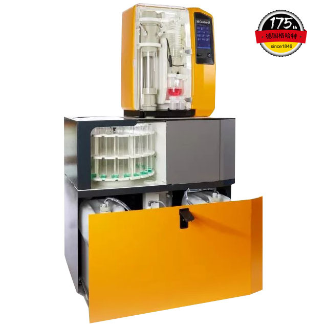
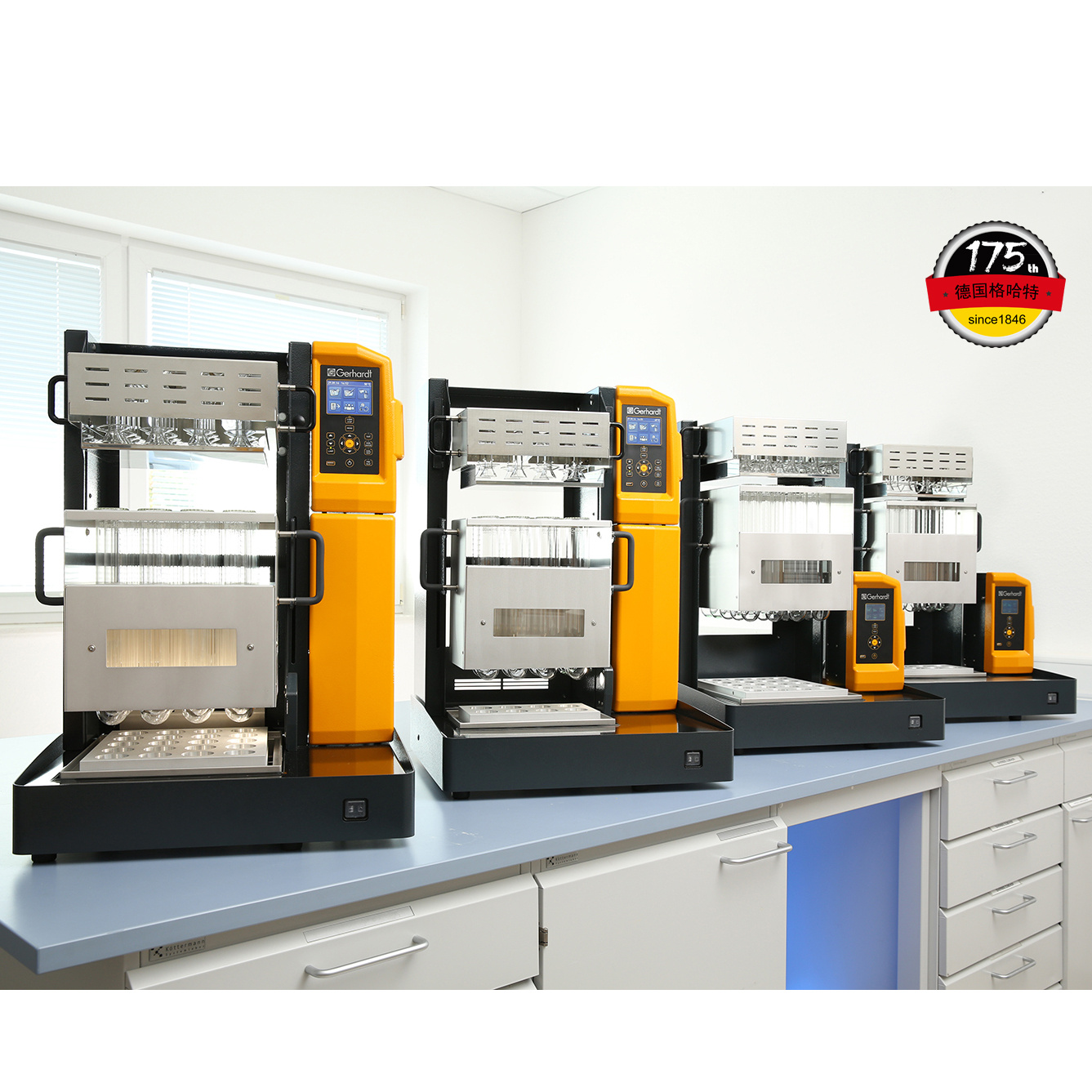
中国格哈特为您提供《玉米、冬油菜和冬小麦田中土壤总氮含量检测》,该方案主要用于其他中总氮检测,参考标准《暂无》,《玉米、冬油菜和冬小麦田中土壤总氮含量检测》用到的仪器有格哈特带自动进样器凯氏定氮仪VAP500C、格哈特凯氏消化系统KT8S、格哈特维克松废气实验室废物处理系统涤气VS、德国加液器MM。
我要纠错
推荐专场
定氮仪、凯氏定氮仪、Dumas定氮仪
更多

相关方案
 咨询
咨询