激波管中密度场和速度场检测方案(流量计)
检测样品
太阳能电池
检测项目
密度场和速度场
关联设备
共3种
下载方案
方案详情文
采用LaVision公司的平面激光诱导荧光(PLIF)系统和粒子成像测速系统(PIV)对2马赫速度激波管进行测量。实验系统由1台Nd:YAG激光器和1台FlowMaster2相机构成。
智能文字提取功能测试中
SANDIA REPORT SAND2011-6497 Unlimited Release Printed September 2011 Experimental Investigation of theRichtmyer-Meshkov Instability Christopher R. Weber Prepared by Sandia National Laboratories Albuquerque, New Mexico 87185 and Livermore, California 94550 Sandia National Laboratories is a multi-program laboratory managed and operated by Sandia Corporation, a wholly ownedsubsidiary of Lockheed Martin Corporation, for the U.S. Department of Energy's National Nuclear Security Administration undercontract DE-AC04-94AL85000. Approved for public release; further dissemination unlimited. Sandia National Laboratories Issued by Sandia National Laboratories, operated for the United States Department of Energy bySandia Corporation. NOTICE: This report was prepared as an account of work sponsored by an agency ofthe UnitedStates Government. Neither the United States Government, nor any agency thereof,nor any of their employees, nor any of their contractors, subcontractors, or theiremployees, make any warranty, express or implied, or assume any legal liability or responsibilityfor the accuracy, completeness, or usefulness of any information, apparatus, product, or processdisclosed, or represent that its use would not infringe privately owned rights. Reference herein toany specific commercial product, process, or service by trade name, trademark, manufacturer, orotherwise, does not necessarily constitute or imply its endorsement, recommendation, or favoringby the United States Government, any agency thereof, or any of their contractors or subcontractors.The views and opinions expressed herein do not necessarily state or reflect those of the UnitedStates Government, any agency thereof, or any of their contractors. Printed in the United States of America. This report has been reproduced directly from the bestavailable copy. Available to DOE and DOE contractors from U.S. Department of Energy Office of Scientific and Technical Information P.O. Box 62 Oak Ridge, TN 37831 Telephone: (865) 576-8401 Facsimile: (865) 576-5728 E-Mail: reports@adonis.osti.gov Online ordering: http://www.osti.gov/bridge Available to the public from U.S. Department of Commerce National Technical Information Service 5285 Port Royal Rd. Springfield, VA 22161 Telephone: (800) 553-6847 Facsimile: (703) 605-6900 E-Mail: orders@ntis.fedworld.gov Online order: http://www.ntis.gov/help/ordermethods.asp?loc=7-4-0#online SAND2011-6497Unlimited ReleasePrinted September 2011 Experimental Investigation of the Richtmyer-MeshkovInstability Christopher R. Weber University of Wisconsin-Madison 1500 Engineering Drive Madison, WI 53706 Abstract The Richtmyer-Meshkov instability (RMI) is experimentally investigated using several differentinitial conditions and with a range of diagnostics. First, a broadband initial condition is createdusing a shear layer between helium+acetone and argon. The post-shocked turbulent mixing isinvestigated using planar laser induced fluorescence (PLIF). The signature of turbulent mixing ispresent in the appearance of an inertial range in the mole fraction energy spectrum and theisotropy of the late-time dissipation structures. The distribution of the mole fraction valuesdoes not appear to transition to a homogeneous mixture, and it is possible that this effect may beslow to develop for the RMI. Second, the influence of the RMI on the kinetic energy spectrum isinvestigated using particle image velocimetry (PIV). The influence of the perturbation is visiblerelatively far from the interface when compared to the energy spectrum of an initially flatinterface. Closer to the perturbation, an increase in the energy spectrum with time is observedand is possibly due to a cascade of energy from the large length scales of the perturbation.Finally, the single mode perturbation growth rate is measured after reshock using a new highspeed imaging technique. This technique produced highly time-resolved interface positionmeasurements. Simultaneous measurements at the spike and bubble location are used to computea perturbation growth rate history. The growth rates from several experiments are compared to a new reshock growth rate model. Contents Abstract..3 Contents5 Figures....6 Acronyms.....7 1.0 Introduction..9 3.1 Background... 3.2 Experimental Setup. 3.3 Interface Characterization. 3.4 Image Processing .... 3.5 Results and Discussion .... Mixing Statistics .... Dissipation Rate. Spectra..... 2.0 Experimental Facility........103.0 Turbulent Mixing in the Richtmyer-Meshkov Instability... .11巧2巧233344 4.0 Influence of the Richtmyer-Meshkov Instability on the Kinetic Energy Spectrum.. 4.1 Background....... 4.2 Experimental Setup... 4.3 Fluctuating Kinetic Energy Spectra... 4.4 Simulation..... .4.5 Summary and Discussion.. 5.0 Richtmyer-Meshkov Instability on a Low Atwood Number Interface after Reshock.. 5.1 Background..... 5.2 Experimental Setup..... 5.3 Experimental Results .. Model Comparison.... 5.4 Numerical Simulation. .6.0 Summary and Conclusion..... 7.0 References.. Distribution....... Figures Figure 1: Diagram of the initial condition setup......... 12 Figure 2: Initial condition image and spectrum...... 1. Figure 3: Initial condition images in the x-y plane.... Figure 4: Spectra in the x and y directions.. Figure 5: Image correction.... Figure 6: Selected images from experimental sequence.. Figure 7: PDF of mole fraction at =0.5. Figure 8: Log of the dissipation rate...... Figure 9: PDF of the dissipation rate.. Figure 10: PDF of the gradient angles....... Figure 11: Light-gas mole fraction energy spectra .. Figure 12: Dissipation spectra ... Figure 13: Initial condition.. ... Figure 14: Post-shocked interface and regions of interest.. Figure 15: PIV results... Figure 16: Particle lag after an impulsive acceleration..... Figure 17: Semi-log plot of fluctuating kinetic energy.. Figure 18:Kinetic energy spectrum at early time.. Figure 19: Kinetic energy spectrum at late time.... Figure 20: Kinetic energy spectra for wave interface.. Figure 21: Kinetic energy spectra for flat interface...... Figure 22: Analysis regions in simulation. .... Figure 23: Kinetic energy spectra from simulation using full domain width..... Figure 24: Kinetic energy spectra from the simulation using the smaller region...... Figure 25: Initial condition image and modal content...... Figure 26: Planar images of the instability...... Figure 27: Experimental x-tdiagram... 巧222333Figure 28: Amplitude vs. time after reshock.3 Figure 29: Diagram of a shock wave passing through a light-over-heavy sinusoidal interface ... 40 Figure 30: Experimental amplitude growth rate divided by the model growth rate.... .....42 Figure 31: Simulation results.. 43 Acronyms CCD Charge Coupled Device DFT Discrete Fourier Transform ICF Inertial Confinement Fusion PDF Probability Density Function PIV Particle Image Velocimetry PLIF Planar Laser Induced Fluorescence RMI Richtmyer-Meshkov Instability RTI Rayleigh-Taylor Instability Experimental Investigation of the Richtmyer-MeshkovInstability 1.0 Introduction The Richtmyer-Meshkov instability (RMI) [1, 2] occurs when a shock wave passes through aninterface separating a pair of gases. Any perturbation on that interface is unstable to the shockacceleration and will grow in amplitude. If the amplitude is much less than the wavelength, thegrowth is linear and given by the equation n=kA*Vno, (1) where k is the wavenumber, A=(p2-p)/(p+P) is the Atwood number, Vo is the velocity ofan unperturbed interface after acceleration by the shock wave, and o is the initial amplitude.The superscript“+”denotes post-shocked quantities. The mixing that results from the RMI becomes important during the compression of an inertialconfinement fusion (ICF) fuel capsule [3], behind the shock wave of a supernova [4], and as amechanism for mixing fuel in hypersonic engines [5]. In all of these applications, knowledge ofhow the instability develops over time and the role certain parameters play in the instability is ofcurrent interest. New insight is gained in this problem through developing models based on well-understood concepts, such as linear stability theory or buoyancy and drag, and comparing theirmodeling of the RMI to experimental and numerical data. Additionally, multiphysics codes usedto simulate high-energy regimes, such as that during ICF or supernova explosion, needexperimental data for validation. Experiments of the RMI provide useful test cases for thehydrodynamic component of these codes. The current work explores three areas where experimental knowledge of the RMI is minimal.The mixing mechanisms inside a turbulent mixing layer are investigated using planar laserinduced fluorescence (PLIF). The influence of the kinetic energy spectrum due to the RMI isanalyzed through particle image velocimetry (PIV). Finally a new technique is introduced tomeasure the growth rate of a single mode interface after reshock. 2.0 Experimental Facility The experiments are performed at the Wisconsin Shock Tube Laboratory [6]. The shock tube is adownward firing, 9.13 m vertical tube. The driver has a circular cross section with a 0.41 mradius and a 2.08 m length while the driven section has a square cross section with 0.25 m sides.A high-pressure boost tank is connected to the driver section by pneumatically-driven fast-opening valves to control the diaphragm rupture time. Piezoelectric pressure transducersmounted along the shock tube side walls are used to trigger the controlling electronics and tomeasure the shock wave speed. Before the experiment begins, the driver is filled to 85%-90% of the diaphragm rupture pressure.The experiment is initiated by opening the fast-opening valve, filling the driver with highpressure gas from the boost tank, and rupturing the diaphragm. The long length of the shock tubeensures a planar shock wave by the time it reaches the interface. Between opening the valves andthe shock wave arriving at the interface, approximately 400 ms has elapsed with a variability ofabout 50 ms. 3.0 Turbulent Mixing in the Richtmyer-Meshkov Instability 3.1 Background Applications of the RMI have initial conditions that consist of a broadband spectrum of modes[7], but the bulk of experimental work has focused on single mode initial conditions. This ispartially because generating a broadband initial condition in the lab is difficult to control. Itrequires either an unknown initial condition [8], a interface that is disturbed by membranefragments [9], or laser-driven experiments with poor spatial resolution [10]. High spatial resolution and knowledge of the initial condition are required to explore the mixingdynamics between the two gases, where gradients in the mole fraction become important. Tounderstand these dynamics, an equation describing the mixing rate can be derived starting withthe continuity equation, We assume the fluid is variable density but incompressible, which is an adequate assumptionafter the shock has passed through the interface. If we nondimensionalize by reference values ofdensity and velocity, we get a nonzero divergence of the velocity [11]: where the Re=UL/v is the Reynolds number,Sc=v/D is the Schmidt number, and D is themass diffusivity. Expanding the continuity equation and using Eq. (3) gives (4) Density can be replaced with the mole fraction, X=(p-p)/(Pz-P), giving 0 Re Sc ReSe1+(n-1)x(vx:vxx) (5) where eta is the density ratio. The right side of this equation is strictly negative and will act toreduce gradients in the mole fraction field, making the flow more homogeneous. To follow alongthe lines of scaling mixing investigations [12-14], this equation can be put in a form similar tothe scalar ‘energy'per unit mass,YX: This is the same as the equation arrived at when starting from the advection-diffusion equationfor a conserved passive scalar, except for the factor on the right: which ranges from 1, where =1, to a maximum of 2 if2>>2. If□1=2, then we are simplytracking the mixing of a conserved passive scalar. The addition of variable density adds weightto dissipation in the higher density areas. In this work, to be consistent with similar work [15],the dissipation rate is referred to as x=DVX·VX. 3.2 Experimental Setup An interface of helium mixed with acetone vapor above pure argon is created 1 m above the endwall of the shock tube. The helium+acetone mixture is made by bubbling helium through twochambers of liquid acetone, the first being heated to 35 C and the second at room temperature.The gas stream is then piped through chilled water so the acetone concentration is slightly belowsaturation and does not condense in the flow-metering equipment. The mixture is at a pressure of50 psi to achieve a sufficient flow rate, resulting in an acetone vapor concentration of 5.3%. Thehelium+acetone mixture is split to the top of the shock tube and to the interface section. Aninitially flat interface is first set up by only flowing helium+acetone into the top of the shocktube and argon into the bottom. Excess gas is evacuated through a pair of vacuum pumpsconnected to slots in the shock tube wall at the interface location. To create a perturbed interface, the helium+acetone mixture and pure argon are injected throughseparate slots into the shock tube. The configuration, shown in Figure 1, was experimentallydetermined to provide the best initial condition in terms of scale and repeatability. Introducingargon above the helium+acetone mixture acts to keep the mixing layer horizontal. Perturbationsappear due to the interaction between the two streams and from the shear between this mixedlayer and the pure argon. In addition to the gas injected at the shear layer, gas is also injected atboth ends of the shock tube. This creates a continual flow towards the interface, ensuring that allof the mixed gas is removed and the mixing layer is steady in time. Figure 1: Diagram of the initial condition setup. Two excimer lasers (Lambda Physik LPX 210i, 308 nm, 470 mJ) are used for planar imaging.The laser beams are combined below the shock tube using a 50-50 beamsplitter and then spread into a sheet with a combination of spherical and cylindrical lenses. A single laser is used for boththe initial condition imaging and a post-shock image, while the other is used for the second post-shock image. Ten pre-shock images are recorded prior to the arrival of the M=1.56 shock waveto obtain a statistical description of the initial condition. To allow the laser to recharge andaccount for variability in experimental timing, the last initial condition occurs around 150 msprior to the shock arriving at the interface. The laser is fired again 0.88 ms after shock arrival tocapture the post-shock interface after it has traveled 26.5 cm. The second laser fires 2.1 ms aftershock arrival, capturing the final post-shock image where the interface has traveled 67.3 cm.Twenty experiments were performed with these settings to obtain an ensemble average.Alternately, five early time experiments were performed where the first post-shock image is stillin the frame of the first camera. The images are all recorded using 3 thermoelectrically cooledAndor CCD cameras. 3.3 Interface Characterization Figure 2(a) shows a sample of the initial condition, corrected so intensity corresponds to relativeacetone concentration or light-gas mole fraction, X. In the image, the gases are injected from theleft near z=0 cm. The pure argon stream is visible above the helium+acetone mixture. Afterabout 3 cm, the two streams of gas begin mixing and the individual streams are no longerapparent. Perturbations develop on the lower edge of this mixing region due to the velocitydifference of the mixture stream and the ambient argon. An additional contour is visible risingfrom the injection location and running horizontally near z =4 cm. This appears to be theboundary between the mixed gas and pure helium+acetone entering from the top of the shocktube. This top contour is diffuse, without perturbations developing on it. Between this topcontour and the bottom shear surface, the average mole fraction is around 0.75. The red dashedlines in Figure 2(a) mark the location where the average mole fraction in the x direction is 0.25,0.5, and 0.75. Figure 2: Initial condition image and spectrum. (a) A sample initial condition image, processed so intensitycorresponds to relative acetone concentration,. The red dashed lines correspond to locations where theaverage mole fraction in the x direction is 0.25,0.5, and 0.75. (b) The mole fraction energy spectra fromlocations denoted in (a), averaged over 40 images. Figure 2(b) shows the energy spectrum of the mole fraction at locations where =0.25, 0.5,and 0.75. These spectra are averages from 40 images. The dashed lines represent a k and kspectra, which roughly match the spectrum at =0.5. These experiments are investigating a 2-dimensional slice in the x-z plane, so it is necessary todetermine how representative this slice is of the whole experiment. To answer this, the initialcondition was imaged in the x-y plane by placing the laser in this plane and positioning thecamera below the shock tube, looking in the z direction. These images allow us to determine ifthe perturbations are 2 or 3 dimensional and if the interface is nearly isotropic in the x and ydirections. Images of the initial condition in the x-y plane are shown in Figure 3 at 6 z-locations, rangingfrom z=2.54 cm to z=-2.54 cm. Gas is injected from the left in these images. At the top of themixing layer, Figure 3(a), there appears to be more mixing features near the edges in the y-direction than in the center. At the next lower plane, the variation in the y-direction is nearlygone. The gradients appear to be sharper towards the left of the image, which is to be expectedsince diffusion and mixing have more time to smooth out gradients by the time the gases reachthe right side. The plane shown in Figure 3(C) is similar to the one above it, with some variationin the y-direction near the left of the image. The bottom two locations seem to be primarilycomposed of ambient argon, with mixed gas entering the plane in the center of the image. >x Figure 3: Initial condition images in the x-y plane. Image planes are located at (a)z=2.54cm, (b)z=1.27 cm,(c)z=0, (d)z=-1.27,(e)z=-1.91, and(f)z=-2.54. Spectra are shown in Figure 4 comparing the spectrum at the center of the image in the xdirection (k. spectrum, region overlaid in red in Figure 3(a)) with the k, spectrum in the ydirection (region overlaid in blue). The spectra are computed using 11 rows or columns of data from each image and from 40 images at each plane. In the image at the highest location, Figure3(a), we saw fewer features in the center of the y-direction than near the edges; the spectra alsoshow this difference, Figure 4(a), with the k. spectrum being weaker than the k, spectrum atmoderate wavenumbers. The next two locations, Figure 4(b,c),have similar spectra at moderatewavenumbers, but at low wavenumbers the k. spectrum is larger. The low wavenumber effect isvisible in the images, as the left of the image appears darker; it is possible that this is due to anonuniform laser beam or a problem in the images correction step. The last three locations,Figure 4(d-f), show very similar spectra for nearly all wavenumbers. It appears that, for a largeportion of the initial interface, the perturbation features are isotropic in the x and y directions. Figure 4: Spectra in the x and y directions. (a-f) correspond to the locations in Figure 3(a-f) respectively. Thelocations where the spectra were computed are shown in Figure 3(a). 3.4Image Processing To translate the raw PLIF images into relative acetone concentration, the images are correctedfor non-uniform laser profile, laser sheet divergence, and Beer’s law attenuation. An uncorrectedPLIF image is shown in Figure 5(a). The general procedure is to transform the image into an r-_coordinate system aligned with the laser beam and correcting for the signal decrease from lasersheet divergence. Then a region in the top of the image is selected where it is assumed a uniformconcentration exists. The exponential coefficient of the signal as a function of r is determinedfrom this region, corresponding to the acetone absorption cross-section, . The normalizedacetone concentration can then be computed [16]: where i(r,) is intensity of a given pixel and io() is the pixel intensity at the top of the image.The image is then mapped back into the x-z coordinate system. Figure 5: Image correction. (a) Uncorrected image and (b) corrected image with intensity proportional toacetone concentration. Some fine-scale features in the top of the laser sheet are not due to the aforementioned effects.As the laser sheet passes through the interface, index of refraction gradients will steer some raysin different directions causing them to not map correctly into the r-coordinate system.Furthermore, the location where they originate can be anywhere within the mixing layer, so theirinclusion in Eq. (8) could introduce unwanted effects into the corrected image. Because of this,high frequency components in the reference intensity io were removed. The two post-shocked image cameras are much slower than the duration of the experiment andare exposed for the entire duration. Because of this, both cameras capture two laser pulses. Thereis no acetone in the frame during the extra laser pulse for the final post-shock exposure, so thisonly adds to the background illumination and is easily corrected. For first post-shocked image,the extra laser pulse illuminates the region far upstream from the interface where theconcentration is uniform. This additional signal is roughly an order of magnitude weaker than thesignal from the desired laser pulse because the laser has attenuated significantly before enteringthe frame, but it still should be corrected for. The region below the interface in the first post-shocked image is assumed to be the constant concentration illumination from the extra pulse.The beam profile is detected in this region along with its spread and attenuation. This profile isthen extrapolated to the full frame and subtracted from the original image. Following this, theabove procedure is followed to determine relative concentration. Figure 5(b) shows the correctedimage with intensity proportional to acetone concentration. 3.5 Results and Discussion Figure 6 shows a sample of corrected images from the experimental campaign. The laser sheet inthe late-time location, near the end wall of the shock tube, is narrower than locations further fromthe end wall, so all images are cropped to the dimensions of the laser sheet in the late-timeimages. The first row in Figure 6 shows three initial condition images. The second, third andfourth rows of images are at post-shock times of 0.14 ms, 0.88 ms, and 2.10 ms respectively.Images in the same column in rows three and four are from the same experiment. Figure 6: Selected images from experimental sequence. First row: initial condition images. Second row: 0.14ms after shock-interaction.Third row:0.88 ms after shock interaction. Fourth row: 2.10 ms after shockinteraction. The width of each image is 8.2 cm. The images show that the large-scale extent of the mixing layer is growing, while the fluidwithin the layer is becoming more mixed and turbulent. The earliest post-shock images seem tohave similar features as the initial conditions, but the gradients are somewhat sharper, likely dueto the compression from the shock wave. The post shock images at 0.88 ms each appear to bedominated by several argon spikes penetrating into the lighter gas. The interface dividing thesespikes from the mixed fluid appears rela1n-tively smooth, without significant secondary Kelvin-Helmholtz instabilities. By 2.10 ms the smoothness along the interface is gone and many small-scale features are present along most contours levels. Mixing StatisticS The large-scale length of the interface is measured by averaging across the width of the image toobtain an average mole fraction profile,(z). The distance between the =0.05 and=0.95 values is used as a measure of mixing layer thickness. An alternate mixing layerthickness, called mixing product thickness h [11], is defined as The three post-shock mixing thickness values are used to estimate the thickness growth rate,giving 24.5 m/s for the =0.05-0.95 definition and 17.0 m/s for the integral definition. Fromthis, the Reynolds number is calculated, Re=hh/v. Table 1 shows the values for mixingthickness and Reynolds number. The Reynolds number is above the proposed threshold for atransition to turbulent mixing, 2x10* [17]. Table 1: Large-scale thickness and Reynolds number Time(ms) h5-95(cm) hp (cm) Re5-95 Re IC 0 6.0±0.5 4.0±0.4 PS1 0.137 3.4±0.2 2.1±0.4 5.55E+04 2.37E+04 PS2 0.881 5.5±0.4 3.0±0.5 8.95E+04 3.36E+04 PS3 2.104 8.3±1.0 5.4±0.9 1.35E+05 6.11E+04 The above definition of mixing thickness does not differentiate between mixed gas and unmixedbut interpenetrating gas. This difference can be expressed in the following ratio [11]: where the denominator is our previous definition of mixing product thickness and the numeratoraverages after converting the mole fraction field into a mix fraction field. This ratio is very highfor the entire experiment, starting at 0.98 for both the initial condition and the earliest post shocktime. For the middle and late post-shock times, the ratio is 0.92 and 0.87 respectively. This trendis comparable to that ofa similar type of flow [18], which finds the mixing fraction start near 1,drop for a short period, and then increase after the turbulent mixing transition to near 0.8. Whilethis ratio is decreasing, the net amount of mixed gas, determined by the numerator, is increasing,going from 2.1 cm at the first post-shock time to 4.7 cm by the third post-shock time. The amount of mixing at the =0.5 location is shown in Figure 7. Initially the mole fraction iswell mixed at this location, with a peak in the distribution around X=0.5. Later in time, thedistribution broadens, spanning over a wider range of mole fraction values. After the transition toturbulent mixing, it has been observed that the distribution becomes more homogeneous with anarrower distribution peak [17-20]. In the current experiments, the growth of large-scaleperturbations introduce unmixed gas into the mixing region, initially reducing the amount ofmixed gas. Viscosity and diffusion will reduce these large-scale perturbations into mixed fluid,which qualitatively appears to be occurring by the latest time images. Experimental measurementat later times than the current ones, which are not possible with the current experimental setup,may see the mole fraction PDF return to a narrow peak. Figure 7: PDF of mole fraction at =0.5 Dissipation Rate The dissipation rate, x=DVx· Vx, is an important factor governing mixing: it provides insightinto the rate at which mixing is occurring and the spatial properties of the mixing structures. Tocompute dissipation, the images are filtered through a 5x5 median filter and the gradientmagnitude is calculated using an 8-point stencil [12]. Figure 8 shows the log of the dissipationrate from the images in Figure 6. The earlier two sets of images show long features stretchingacross the width of the image. At the time of the second post shock image, the structures arebecoming more vertical as the heavy spikes protrude into the mixing layer. By the latest time, themixing structures appear very chaotic without an obvious preferred direction. Vertical lines arepresent in the images above and sometimes below the interface. These are artifacts fromdistortions in the laser sheet that were not removed in the image processing step. To avoidcounting these artifacts and limit the effect noise has on the statistics, a mask is applied to theimages, keeping information only in the region 0.1=0.5 location. Five rows oneither side of the row nearest to =0.5 are used to produce an average spectrum from eachexperiment. The spectrum from each row is interlaced with the neighboring row to reduce theeffect of noise at high wavenumbers [22]. The average spectra from the 4 times are shown inFigure 11 with compensated spectra shown in Figure 11(b). Figure 11: (a) Light-gas mole fraction energy spectra and (b) compensated spectra at =0.5. It is possible that an inertial range is developing in the late time spectrum between k=1.5 cmand 8 cm, as this region is nearly flat in the compensated spectrum of Figure 11(b). Thedissipation spectra, D=kE, are shown in Figure 12. The Batchelor length scale can be estimatedfrom the dissipation spectrum as the scale where the spectrum is 2% of the maximum [23].Figure 12(b) is normalized to the maximum dissipation and a dashed line is showing the 2%level. The 2% level for the latest time experiments can be discerned,showing scale of 950 um. The spectrum of the earlier time experiments in Figure 12(b) becomes noisy at highwavenumbers near the 2% level, but it appears that the 2% scale would have been smaller thanthe later time scale, possibly around 730 um. An increase in the Batchelor length scale with timeis what we anticipated earlier from the scaling argument, ag~8Re-34 Sc-12. Figure 12: (a) Dissipation spectra and (b) normalized dissipation spectra with a dashed line representing the2%level. 4.0 Influence of the Richtmyer-Meshkov Instability on the KineticEnergy Spectrum 4.1 Background RMI studies typically investigate the growth of the perturbation (for examples, see the reviewarticle by Bouillette [24]). Some effort has been made to study the turbulence that results fromthis perturbation growth. Laser doppler anemometry measurements have characterized thefluctuations inside the turbulent mixing zone, where dissipation and diffusion reduce themagnitude of the fluctuations but expand the spatial extent of this zone [25]. The mixing withina shocked gas-curtain showed that a late time transition to Kolmogorov scaling occurs [24,25].The energy transfer within the Rayleigh-Taylor instability (RTI) was studied through directnumerical simulations [28], showing that energy is initially concentrated in scales correspondingto the dominant wavelength and spreads out to larger wavenumbers as vortex stretching andbending transfer energy to smaller scales. A description of the energy scales in the RMI and how they vary in space and time is importantto applications in inertial confinement fusion (ICF) and shock-induced mixing from supernovaexplosions.Simulations in these areas often use subgrid-scale models [27,28] to approximate theenergy transfer to and from unresolved scales. These models rely on coefficients that need to beset to provide the best description of the underlying physics. An additional consideration,particularly in ICF, is the far-field effect of the instability. If the presence of a perturbation on theinterface is felt far from the interface, it can have an influence on fusion ignition and burn wavepropagation. This influence begins with the distorted transmitted shock wave converging to thecapsule center. When the shock wave passes from a light gas to a heavy gas, a reflected shock wave willpropagate away from the interface through the light gas. This reflected shock wave initially takeson the distorted shape of the perturbed interface and, as it returns to planar, will leave a wakebehind. This occurs because the concave portion ofthe distorted shock wave will convergeslightly and strengthen. With the two refracted (transmitted and reflected) shock waves, theeffect of the interface is felt far from the interface. The interaction of the shock wave with the gas far from the interface can be described as beingsimilar to the shock-turbulence interaction, where a shock wave passing through a turbulent fieldwill amplify any existing turbulence in the flow [31]. In RMI experiments, any backgroundturbulence present in the shock tube will also be amplified. In addition, the shock will interactdifferently with the longitudinal and transverse components, leaving behind an anisotropicturbulent field. After the interaction, without any additional production of turbulence, theturbulence will return to isotropic and decay through dissipation [23]. Additional production of turbulence, however, can be found near the interface of the RMI. Aturbulent viscosity model [23] has the production term The velocity gradients from the interfacial perturbation growth act as a source of turbulence thattransfers to smaller length scales. The fluctuating kinetic energy spectrum initially containsenergy at the large scales approximately equal to the wavelength of the perturbation. After sometime, the spectrum will have filled out to the inertial sub-range, and then to the dissipation range.Cook and Zhou [28] described the energy spectrum in the RTI and showed that the dominantwavelength initially had the bulk of the kinetic energy, but as the instability developed thespectrum filled out to larger (due to bubble merger) and smaller scales. The main differencebetween the energy in the RTI and the RMI is that the former is continuously forced by thesustained acceleration field while the latter only has the energy left behind by the shock wave. The perturbation growth and the interaction of the distorted shock wave with the surrounding gasleads to several turbulence mechanisms operating at different scales, locations, and times. Thework discussed here analyzes the energy spectra at two times and at two locations with respect tothe interface. The location further from the interface is considered similar to that of the shock-turbulence interaction, where dissipation and return to isotropy are the two processes that can beexpected to occur. The turbulence at the location near the interface is expected to experience theadditional production mechanism of the RMI perturbation growth. 4.2 Experimental Setup AN2-SF6 interface is created by flowing N2 from the top of the shock tube and SF6 from thebottom. Slots, located 1 m from the bottom of the shock tube, allow a stagnation plane to formand excess gas to be removed with the aid of a vacuum pump. The slots are centered in a pair of5.08×25.4 cm" rectangular pistons that are embedded in the wall of the shock tube wall. After thegases have flowed for a sufficient time to ensure purity, the pistons are oscillated at 3.27 Hz for10 revolutions to create a 2-dimensional standing wave with an initial amplitude of 0.38 cm anda wavelength of 9.1 cm. An example of this initial condition is shown in Figure 13. The Atwoodnumber of the interface is 0.68 initially and 0.77 after being compressed by the shock wave. 一E> Figure 13: Initial condition. The N2-SF6 interface with the waveform initial condition is shown just prior tobeing accelerated by a shock wave. The N2 is seeded with Al2O particles. Prior to the experiment, the driver section is filled to 90% of the diaphragm rupture pressure.Excess pressure is then released into the driver using fast-opening valves that are timed inrelation to the standing wave, rupturing the diaphragm and launching a shock wave towards the interface. The shock wave has an incident Mach number of M=2.05 and the post-shockedinterface velocity is 298 m/s. Flow visualization is performed by seeding the N2 with Al2O3 particles using a TSI fluidized bed(model 3400). Particles are mixed with the flow for approximately a minute prior to theexperiment, allowing for a uniform particle distribution to be observed. Planar images areobtained using two lasers and three cameras. The initial condition is illuminated using acontinuous Ar laser of approximately 1W in power and spread into a sheet with a cylindricallens. A high speed camera, IDT model XS4, is set up at the location of the stagnation plan torecord the standing wave being created and determine the final interface shape before the shockreaches the interface. The post-shocked interface is recorded using two cameras and a dual-cavity Nd-YAG laser. The two pulses from the Nd-Yag laser are spaced 14 us apart and have apulse duration of~10 ns. A LaVision Flowmaster 2 camera is focused onto a 2.2 cm x 2.8 cmregion and records two images corresponding to each of the Nd-YAG pulses. Athermoelectrically cooled Andor CCD camera is mounted at an angle to the image plane toaccommodate the LaVision camera, and provides a full-field view of the interface. The slowshutter on this camera requires that both Nd-YAG pulses are captured on a single image. Bothcameras have a 532 nm laser line filter to allow only the light from the Nd-YAG laser. Images obtained from two experiments are shown in Figure 14; each image was taken with thefull-field camera and the rectangular boxes show the regions that the zoomed-in camera isfocused on. The obstruction in the right half of the image is the LaVision camera. These imagesare taken at 0.3 ms and 1.0 ms after the shock wave accelerates the interface and the locations are5 cm and 9 cm away from the interface at both times. Figure 14: Post-shocked interface and regions of interest. These images are taken with the full-field camera at0.3 ms and 1.0 ms showing the post-shocked interface with an initial waveform perturbation. The blue boxesshow the regions that the PIV camera (black obstruction in the right half of the image) is focused on. The pair of zoomed-in images is analyzed using particle image velocimetry (PIV) to obtain avelocity field. The mean flow has displaced 200 pixels between the two images, allowing smalldifferences in the velocity field to be measured. The first step in the PIV analysis is to removethe background by subtracting a median filtered image from the original image. The backgroundsubtraction helps remove a zero-displacement bias of the cross-correlation procedure. The two images are shifted by the estimated mean displacement and a cross-correlation analysis is appliedto 64x64 pixel regions across the image to obtain the displacement field. The sub-pixeldisplacement is determined by assuming the cross-correlation matrix has a Gaussian shape andinterpolating to find its peak location [32]. The displacement field is then filtered to removespurious vectors and smoothed. The two images are then deformed using this displacement fieldand a bilinear interpolation algorithm. The first image is deformed by half the displacement fieldand the second is deformed in the opposite direction by half the displacement field, ideallyresulting in two images with identical particle locations. A cross-correlation analysis is thenapplied to the deformed image. This process of image deformation and cross-correlation isiterated, without the smoothing step, until the deformed images have a negligibly smalldisplacement field. This iteration occurred four times with a decreasing window size andincreasing overlap, reaching a final size of 32x32 pixels with 50% overlap. This iterative imagedeformation method has been shown to improve the precision of sub-pixel displacementmeasurements by an order of magnitude over cross-correlation met?1hods without imagedeformation [31,32]. An example of a velocity field from PIV is shown in Figure 15(a) from a late time image farfrom the interface which corresponds to the upper rectangular box in Figure 14(b). The meanvelocity of 298.2 m/s is removed, showing the fluctuating field. A reference vector of 5 m/s isshown in the upper right of the image and Figure 15(b) shows the magnitude of the velocity. Thespatial resolution of the velocity field is 335 um. The turbulent intensity, defined as U averaged over all of the experiments is 0.59% in the streamwise direction and 0.87% in thetransverse direction. A conservative estimate of PIV measurement error of 0.1 pixeldisplacement would correspond to 0.15 m/s which would change the turbulent intensity by0.05%. Figure 15: PIV results. (b) The vector field from a PIV analysis with the mean velocity subtracted. Thereference vector in the top right corner is 5 m/s. The background is the original particle image. (b) Thevelocity magnitude of the image in (a). The second source of error comes from the ability of the particles to track the flow. The particleshave a stated size of 50 nm but may agglomerate to sizes much larger than this [35]. A way ofindirectly determining the particle size is by observing the lag distance behind the flow. Figure16 shows an experiment where the bottom gas was seeded and the shock wave impulsivelyaccelerated the interface to 390 m/s. The image shows that, while there are a handful of particlesthat fell behind the interface by ~1 cm, the majority of the particles are within 0.25 cm of theinterface. Using this distance in a Stokes drag calculation, a particle size of 1.1 um is found.Hjelmfelt and Mockros [36] analyzed the ability of a particle to follow the turbulence of a givenfrequency.With this particle size, a maximum turbulence frequency of 27 kHz is observable.From the eddy turnover frequency, uyk/2n, obtained from the energy spectra data that will bediscussed below, a maximum turbulent frequency of~200 Hz is observed. Therefore theseparticles adequately follow all eddies in the post-shocked flow. x(cm) Figure 16: Particle lag after an impulsive acceleration. The initially flat interface was shock-accelerated to390 m/s and some particles required a distance to accelerate to the gas velocity. Some particles are up to 1 cmbehind the interface, while the majority of the particles are within 0.25 cm. 4.3 Fluctuating Kinetic Energy Spectra The spectrum of turbulent kinetic energy is computed in both thex(transverse) and y(streamwise) directions. The procedure for the x-direction is as follows. The fluctuating velocitywithin a row of the velocity field data is obtained by subtracting off the mean velocity in thisrow. A discrete Fourier transform (DFT) of the fluctuating velocity is computed using a windowfunction to reduce spectral leakage [37]. As in other experimental turbulence spectrameasurements [36,37], a Hanning window function was chosen for computing the DFT. Thetotal kinetic energy spectra are found by multiplying the transformed component by its complexconjugate and adding the energy from the other direction of velocity. An example of this energyspectrum is shown in the semi-log plot Figure 17, where the x-axis is the log of the wavenumberand the y-axis is the location of each row. This plot shows that the spectrum does changesignificantly throughout the domain. Each spectral component is averaged across the domain andcombined with that of two other experiments of the same type (same time, location, and initialinterface). Figure 17: Semi-log plot of fluctuating kinetic energy. The y-axis is the physical dimension in the PIV imageand the x-axis is log of the wavenumber. The energy spectrum does not change significantly throughout theheight of the domain. As already mentioned, data is taken at two times, referred to as early and late, and at twolocations, referred to as near and far with respect to the interface. The experiments are conductedwith an initial sinusoidal waveform imposed on the interface and with an initially flat interface,referred to as wave and flat experiments, respectively. Three experiments were conducted foreach of these eight different scenarios, with a total of 24 experiments in all. The spectra shown inthe following figures are averages from the three experiments. Figure 18 shows the fluctuating kinetic energy spectra at the early time. The error bars representthe 95% confidence interval for the mean energy at that wavenumber across the entire velocityfield from the three experiments of the same type. For most wavenumbers in the spectra, the k,modes have a higher energy content than the k. modes. This is true for both the initially flatinterface and that with a waveform perturbation. This shows the anisotropy of the post7-5/3-shockedturbulence. Because the turbulence is anisotropic, we do not expect a kscaling. The spectrahave a slightly lower slope than -5/3 up until about 4x10'm, after which the slope is steeper, possibly signifying the beginning of the dissipative range. Since the initial turbulence spectrum isnot known, the anisotropy may be due to the shock wave or the initial spectrum. Near the interface in these early time experiments, the first few lower wavenumber modes in thek. direction have a higher energy content when the waveform is present on the interface. In the k,direction, and at higher wavenumber in the k direction, the flat interface spectra have a slightlyhigher energy content when compared to waveform experiments. The reason for thesedifferences is not clear. Further from the interface the spectra from the interface with an initialwave perturbation have a higher energy content than that of the initially flat interface. A possibleexplanation for this is that the region further from the interface has more recently experienced ashock wave passing through it. The shock wave that reflects off the interface is deformed with ashape similar to the interface and distorts the flow field behind it as it returns to planar. The nearlocation has had more time for these effects to dissipate away. It can also be seen that the spectraat the far location are larger in magnitude than that of the near location at this early time, whichalso suggests that dissipation is behind these differences. From this, we can expect that thedifferences in the far location will become less at later times. Figure 18: Kinetic energy spectrum at early time. (a) Location near and (b) far from the interface for both aninterface with a waveform perturbation and a flat interface. The error bars signify the 95% confidenceinterval for the mean values. The fluctuating kinetic spectra for the later time experiments are shown in Figure 19. In Figure19(b), we see that, as expected, the differences in the kinetic energy spectra are reduced: thespectra from the experiments with an initial wave are nearly the same as that from the flatinterface experiments. The k, spectra are still larger than the k. spectra so it appears that a returnto isotropy will occur at larger times scales than are observed between these experiments. At thenearer location the spectra for the wavy interface in both directions are larger than those for theflat interface. The spectra in Figure 19(a) do not extend to the high wavenumbers that areobtained in the rest of the experiments because the PIV interrogation window size was doubled.At this location it appears that mixing between the two gases and boundary layer effects arecausing refractive index gradients, known as aero-optical effects [40],to blur the image slightly,so a larger interrogation window was needed to include enough clear particles to get an accuratevelocity measurement. Figure 19: Kinetic energy spectrum at late time. (a) Location near and (b) far from the interface for both aninterface with a waveform perturbation and a flat interface. The change in the spectra over time is shown by combining Figure 18 and 7. Figure 20(a) showsthat near the perturbed interface, the spectra at higher wavenumbers increase in energy contentbetween the early and late times. At the location further from the interface, Figure 20(b), theenergy content at all wavenumbers decreased from the early to the late time. These spectra seemto confirm our hypothesis, that the deforming interface will add kinetic energy near to it, whiledissipation will dominate further from the interface. Near the flat interface, Figure 21, the energy spectra stay nearly the same, decreasing slightly fora few wavenumbers. Far from the flat interface the spectra also stay roughly the same; the k.spectra increases slightly at high wavenumber and decreases slightly at low wavenumbers. It wasexpected that a decrease in the energy spectra would have been observed in these figures, similarto that of Figure 20(b). What appears to be occurring is that the excess energy left behind by thedistorted shock wave is quickly dissipated away. This rate of energy dissipation is higher thanthe dissipation of the initial turbulence, which is presumably present in the flat interface spectraand does not change significantly. Figure 20: Kinetic energy spectra for wave interface. The spectra at different times are compared at the (a)near and (b) far locations. Figure 21: Kinetic energy spectra for flat interface. The spectra at different time are compared at the (a) nearand (b) far locations. 4.4 Simulation To confirm the trends discussed in these experiments, a single mode, two-dimensional simulationwas preformed. The initial conditions in the simulation were set to match the initial Machnumber, wavelength and amplitude of the experiment. No initial velocity, other than the shockedgas, was present in the initial setup. The simulation uses 10th order spatial differencing with a4th order Runge-Kutta temporal integration. An artificial fluid large eddy simulation (LES)scheme is used to provide stability along with the appropriate numerical dissipation [41]. Theresolution in the simulation is /256=348 um, providing a similar resolution to the PIV data. The fluctuating energy spectra are computed in regions chosen to be a similar distance from theinterface as the locations observed in the experiments. The red region in Figure 22 spans theentire width of the domain. Since the x-boundaries in the simulation are periodic, the spectra inthis region can be computed without the use of a window function. The green region is chosen tobe the same size and location as in the experiments, but it is necessary to use a Hanning windowfunction when computing the DFT. Figure 22: Analysis regions in simulation. A field plot of N2 (black) and SF6 (white) is plotted from thesimulation at 0.9 ms and the two analysis regions are shown. The Fourier transform in the full width of thedomain (red) allows us to take advantage of the periodic boundary conditions. The green region is chosen tomatch the region investigated in the experiment. Figure 23 show the spectra computed using the full width of the domain. The trends of interest inthese spectra are an increase in spectral energy at the near location and a decrease in energy farfrom the interface. These trends appear to be present for most wavenumbers. A hump in thespectrum is present at the earliest time near k=2000 mat both locations and dissipates away.It is not clear where this feature comes from. Since the simulation is 2-dimensional, a kspectrum is expected for fully developed turbulence [42] and is observed at the later time nearthe interface. Figure 23: Kinetic energy spectra from simulation using full domain width. Five energy spectra are plottedfrom different times to show changes (a) near and (b) far from the interface. Figure 24 shows the spectra computed within the green box in Figure 22 and using a Hanningwindow function. Near the interface at this location the energy spectra decrease for the first fewtime steps and then increase over the last three time steps. The hump in the spectra is also presentat this location and is gone by the later times. Further from the interface, nearly all modesdecrease in energy at each time step. Figure 24: Kinetic energy spectra from the simulation using the smaller region. The smaller region of interest(a) near and (b) far from the interface is chosen to match the location observed in the experiments. Theenergy spectra from five times are shown. The simulation data appear to confirm the results shown in the experiments, that energyproduction occurs near the interface and dissipation dominates further from the interface. A 3-dimensional simulation is necessary to make quantitative comparisons to the experiments, as thephysics of the energy cascade are fundamentally different in three dimensions. At the presenttime, a 3-D simulation has not been computed because of the significant computational costrequired to resolve the necessary scales. 4.5 Summary and Discussion This work investigated the energy spectra at small scales in the presence of a shock-acceleratedinterface and the effect that the Richtmyer-Meshkov instability has on the spectra. It is observedthat, near the perturbation, the energy spectra increase in time as energy from the large scales ofthe perturbation cascades towards smaller scales. Further from the interface the presence of theperturbation is observed, as the fluctuating kinetic energy is higher than that of a flat interface.Later in time these differences are no longer present, as dissipation has reduced the excessenergy deposited by the distorted reflected shock wave. It is unclear as to why the spectra with a flat interface stay largely unchanged between the twotimes. It is possible that dissipation effects will be enhanced and more easily observed in a flowwith higher turbulence intensity. When the flow becomes isotropic is not known and experimentslater in time are needed to investigate this. This is, as far as the author is aware, the first time that the influence of the RMI on the kineticenergy spectrum has been experimentally investigated at different locations from the interface.Since this influence extends beyond just the mixing region, it is possible that applicationsconcerned with the RMI will need to consider more than just the mixing width. 5.0 Richtmyer-Meshkov Instability on a Low Atwood Number Interfaceafter Reshock 5.1 Background An interface between two gases that is accelerated by a shock wave is unstable regardless of thepath the shock wave takes. If the shock wave travels from the light gas to the heavy one,perturbations on the interface will grow in amplitude. If the shock travels in the reverse direction,the vorticity will be of the opposite sign than the previous case, and the perturbation will firstcompress and reverse phase, and then grow in the opposite direction. These cases can becombined in a shock tube by allowing a once-shocked interface to be reshocked by a shock wavethat reflects from the end wall. Shock tube experiments investigating the RM instability after reshock have the advantage thatthe interface is nearly stationary after reshock, allowing the interface to be viewed in the samewindow for a longer period of time. At the time of reshock, the interface has grown in amplitude.When the reflected shock wave passes through this larger interface, the vorticity deposited willbe much larger than that from the first shock interaction. The larger vorticity will cause theamplitude growth rate after reshock to be several times larger in magnitude than prior to reshock. Previous shock tube experiments investigating the RM instability after reshock have obtainedfull field images using either planar imaging [16,41] or schlieren [22,42]. The amount of datacollected for each experiment is limited by the laser pulse rate or the camera frame rate. Thecurrent work uses two continuous laser beams to acquire high speed amplitude measurements.This new method has two advantages: data can be taken with higher temporal resolution and themeasurements are taken from the same plane as the planar imaging. The experimental results arecompared with models and a simulation. Additionally a new model is introduced for circulationand amplitude growth rate estimates for single or multiple shock waves. 5.2 Experimental Setup The interface is created in the shock tube by flowing pure argon gas from below and a 50-50%volume fraction mixture of helium and argon from above [45]. The gases meet to form astagnation plane and exit through slots in the shock tube due to a pressure differential providedby a vacuum pump. The slots are centered in a pair of 5.08×25.4 cm rectangular pistons that areembedded in the walls. After the gases have flowed for a sufficient time to ensure purity, thepistons are oscillated at 1.25 Hz for 14 rPisevolutions to create a standing wave with an initialamplitude of 0.35 cm and a wavelength of 19.4 cm. The interface has an Atwood number(4=(-r)/(r+r)) of 0.29. A sample initial condition image is shown in Figure 25 along witha modal decomposition, showing that the perturbation is primarily a single mode. Figure 25: Initial condition image and modal content. L,is the streamwise region of interest for the initialcondition and L is the spanwise dimension. Before the experiment begins, the driver is filled to 85% of the diaphragm rupture pressure.Approximately 300 ms before the acceleration of the desired standing wave occurs, a high-pressure boost tanks opens, filling the driver with gas, and rupturing the diaphragm. The longlength of the shock tube ensures a planar shock wave by the time it reaches the interface. Theincident Mach 1.92 shock wave transmits through the interface and reflects from the end wall asa Mach 1.70 shock wave. Flow visualization is performed by seeding the bottom gas with Al2O3 particles using a fluidizedbed. Four lasers enter from the bottom of the tube, illuminating a plane halfway between thefront and back walls. Planar images are acquired using a KrF excimer laser for an initialcondition image and a dual cavity Nd:YAG laser for post-shocked/re-shocked images. The initialcondition image is recorded on a cooled Andor CCD camera and a pair of post-shocked or re-shocked images are captured with a Lavision PIV camera. In addition to planar imaging, a high speed diagnostic is implemented using two continuousargon ion laser beams entering from the bottom of the tube and positioned below the spike andbubble of the initial condition. The Mie scattering signals from the laser beams are recorded withtwo high speed cameras from Redlake and IDT at 116,509 Hz. The data from these cameras areused to track the transmitted and reflected shock waves and observe the interface as it travelsthrough the viewing window. This setup allows for an experimental x-t diagram to beconstructed from each camera. Amplitude growth over time can then be determined using the x-tdiaphragms from the two cameras. 5.3 Experimental Results A set of planar images is shown in Figure 26. The first image is taken 0.10 ms before thereflected shock wave has reached the interface. The interface has grown to 0.92 cm in amplitude.The first image shows a few stray particles up to a centimeter above the interface. The seedingmethod allows for a distribution of particles of various sizes, with larger particles taking longerto accelerate in the presence of high velocity gradients, such as the passage of the incident shockwave. The maximum particle size is estimated to be 2.1 um. This value is calculated using thedistance lag of the particles in Figure 26(a) and the velocity of the interface [35]. The definedcontour of the interface suggests that most particles are of sufficiently small size to show no lag. The images after reshock, Figure 26(b)-(h), initially show the interface compresses in amplitudeat 0.06 ms and then reverses in phase by 0.61 ms. Later in time, after 0.86 ms, secondary instabilities can be seen arising on the interface, predominantly at the mid location between thespike and the bubble. The rarefaction that reflects from the end wall is expected to be arriving atthe interface after the 0.86 ms image. (a) (b) (c) (d) (e) (f) (g) (h) Figure 26: Planar images of the instability. Image (a) was taken 1.86 ms after being accelerated by the firstshock wave but 0.10 ms before being reshocked. The following images all occur after being reshocked withthe time after reshock being (b) 0.06 ms, (c) 0.34 ms, (d) 0.61 ms, (e) 0.86 ms, (f) 1.09 ms, (g) 1.34 ms, and (h)1.63 ms. (a) (b) Figure 27: Experimental x-t diagram from an (a) initially flat interface showing the scattered light signal,revealing the transmitted and reflected shock waves and the path of the interface. (b) Experimental x-tdiagrams showing the interface location for a bubble (blue) and spike (red) from a single experiment. Alsoplotted is the interface location from an initially flat experiment (black). Figure 27(a) shows an example of an experimental x-t diagram taken from an initially flatinterface. In the beginning (tr~-2 ms), unshocked seeded argon can be seen. At tr~-1 ms thetransmitting shock can be seen traveling through the diagram, where it compresses the seededargon, causing the scattered signal to intensify. At tr~0.5 ms the interface travels through thediagram until it is reshocked at tr=0 m and 78 cm from its initial location. The reshockedinterface then travels upward in the tube (to the left in the diagram) until the rarefaction wavethat reflects off the bottom wall causes the interface to become nearly stationary. At tr~0.6 msthe pulse from the Nd:YAG laser can be seen. At tr~ 3.5 ms a wave that has reflected off thecontact surface between the driver gas and the driven gas causes the interface to movedownward. Figure 27(b) shows the locations for a spike and bubble from a single experimentcompared with that from an initially flat interface experiment. Model Comparison Amplitude vs time after reshock of six experiments are extracted from the experimental x-tdiagrams and plotted in Figure 28. The differences in initial condition amplitudes resulted in theamplitude before reshock to range from 0.82 cm to 1.76 cm. The variation in the amplitudegrowth rates due to the different initial conditions allows for a comparison to several reshockgrowth rate models. Brouillette and Sturtevant [46] extended Richtmyer’s impulsive model: 7=knAvA* (16) to include multiple shock interactions through a summation of the impulsive growth of each: 4 Figure 28: Amplitude vs. time after reshock for six experiments. The amplitude before reshock is 0.82 cm(black), 0.97 cm (blue), 1.05 cm (magenta), 1.33 cm (cyan), 1.48 cm (red), and 1.76 cm (green). Mikaelian [47] extended the phenomenological model of the Rayleigh-Taylor mixing layerexperiments and simulations of Read [48] and Youngs [49] to the Richtmyer-Meshkov instabilityafter reshock: n=0.14AvA*. (18) Although this model describes three-dimensional multimode interfaces, it has been shownpreviously to provide a good estimate of amplitude growth of single mode interfaces afterreshock [50]. Jacobs and Sheeley [51] showed that for a low A interface the circulation on a half-wavelength is related to the amplitude growth rate by n - - a (19) We use this relation with a model estimating the circulation deposited on the interface to producea new growth rate model. The velocity field around the interface as the incident shock isrefracting can be approximated by dividing the region into the corresponding values calculatedfrom one-dimensional gas dynamics, shown in Figure 29(a). The circulation deposited on theinterface can be modeled by performing a line integral about a closed contour, P, forming a boxaround a half-wavelength: This line integral, shown in Figure 29(a), becomes where (a) (b) Figure 29: Diagram of a shock wave passing through a light-over-heavy sinusoidal interface. (a) Single shockinteraction: incident shock wave is propagating downward through an unshocked interface. (b) Reshockinteraction: reflected shock wave is traveling up through the once-shocked interface. The time is taken to be the time it takes for the incident shock wave to travel across the entireinterface, i.e. t=2n /W. Combining Eqs. (19) & (20), and noting that u,=0, yields an estimate forthe growth rate due to the incident shock wave. A similar approach is applied to the reshocked interface, shown in Figure 29(b). In this case, thewave reflects off the interface as a rarefaction wave, which we can estimate to be traveling at thesound speed in that medium. The line integral becomes where. We can simplify these equations by noting that u=0. The signs of all velocities are taken to bepositive downwards in Figure 29(a,b). Since the vorticity from the two interactions will add tothe net circulation, the two growth rates should be added to provide the net growth rate afterreshock. The final growth rate after reshock is The experimental growth rates divided by the growth rate predicted by each of the models areshown in Figure 30. The time is scaled by the wave number and the model growth rate. Figure30(a) uses the growth rate determined by the Brouillette and Sturtevant model, Eq. (2).Reshockoccurs at t=0 and the rarefaction wave that reflects offthe end wall interacts with the interfaceat t ~0.3. At a time halfway between the reshock and rarefaction, the model underestimates thegrowth rate on average by 59%. It is interesting to note, however, that the growth rate of only theinteraction of the second shock, shown in Figure 30(b), does accurately describe the growth rateof the experiments after reshock by overestimating the growth by only 7%. The model growthrate from the Mikaelian model, Eq. (18), is used in the scaling of Figure 30(c). Here we find themodel does not collapse the growth rates well, but it does roughly match the growth rate of theaverage of the experiments. The average growth rate is overestimated by 12%. The 1-Dcirculation based growth rate model, using Eq. (22), is used in the scaling of Figure 30(d). Themodel overestimates the growth rate on average by 19%. It performs best when the amplitudebefore reshock is larger: for the 7or=1.75 cm experiment, the model was above theexperimental growth rate by 2%. 4 4 (c) (d) Figure 30: Experimental amplitude growth rate divided by the model growth rate. The model growth ratesused are from (a) the Brouillette-Sturtevant model, (b) the impulsive model using only reshock, (c) theMikaelian model, and (d) the 1-D circulation based model. The models vary in their ability to collapse the experimental growth rate to a single curve. Themaximum difference in the normalized growth rates between the different experiments is largest for the Mikaelian model at 0.90. This model does not contain a parameter for the initialamplitude, so experiments with high initial amplitude are growing faster than the model and theopposite for smaller initial amplitude experiments. The Brouillette and Sturtevant modelcollapses the experimental data better, with a maximum difference in normalized growth rate of0.49. The 1-D growth rate model provides the best data collapse, with a maximum difference innormalized growth rate of 0.30. 5.4 Numerical Simulation A numerical simulation of the average experimental conditions was performed using thehydrodynamics code Raptor, developed at LLNL, that solves the 2-D compressible Eulerequations on a fixed (Eulerian) grid. The shock-capturing scheme uses a higher order Godunovsolver to handle the shock propagation and suppress spurious oscillations near the discontinuity.Two levels of adaptive mesh refinement are applied to density gradients and along the interfacewith ratios of 4 and 4. The finest resolution has 512 cells per shock tube width (0.50 mm/cell). The initial condition is a single mode sine wave based on the average amplitude and wavelengthof the experiments. The interface was given a hyperbolic tangent diffusion thickness to match thecalculated value of 1.42 cm [45]. The domain is initialized from the stationary state to capture allshocks and waves that arise during the experiment. The amplitude growth rate from the simulation is compared with that from an experiment with asimilar initial condition in Figure 31(a). The growth rate after reshock and after the reflectedrarefaction are nearly identical, while the growth rate during the reflected rarefaction peakshigher for the experiment, both the simulation and experiment show the same trend. The 1-Dmodel overestimates the growth rate after reshock of the simulation by 7%. t, (ms) Figure 31: Simulation results comparing (a) the amplitude growth rate from the simulation (black) with thatfrom a similar experiment (red) and the 1-D model (dashed). (b) Circulation over a half wavelength from 1-Dmodel (dashed) and the simulation:+(solid-blue),.(solid-red), and net (solid-black). The results of the simulation allow for a direct comparison between the circulation from the 1-Dmodel and that in the simulation. The circulation over a half-wavelength is integrated from thevorticity field and plotted in Figure 31(b). The net circulation of the simulation is initially withinabout 2% of the circulation predicted by the model after the first shock. As the instabilitydevelops further in time the circulation becomes about 30% less in magnitude than the modelprediction. After reshock the circulation initially is within 3% of that predicted by the model andbecomes underestimated by about 40% as the instability develops in time. The model onlypredicts the initial baroclinic circulation deposition, so the drop in the magnitude ofthecirculation as the instability develops in time is not expected to be reproduced by the model. Thefact that the amplitude growth rate predicted by the model is higher than that seen in the experiment and simulation suggests that this reduction in circulation could be an importantparameter in the amplitude growth rate. 6.0 Summary and Conclusion A statistically repeatable broadband initial condition was created for the Richtmyer-Meshkovinstability. The initial condition is free of any interference from membrane or other physicalobstruction and allows for high resolution imaging of the mixing structures within the turbulentmixing layer. When accelerated by a M=1.56 shock wave, the helium+acetone over argonmixing layer exceeds the transition to turbulent mixing threshold of Re=2x10*. Qualitatively,turbulent mixing appears to be occurring by the latest time images, but PDFs of mole fraction donot show a more homogeneous mixture. It is possible that the interface needs more time totransition than available in these experiments. The energy spectrum at the late time appears toshow evidence of an inertial range and PDFs of the angle of the mixing/dissipative structuresshow that the mixing layer is nearly isotropic by the late time. The measurements of turbulent kinetic energy showed that the perturbations influence thespectrum a relatively far distance from the interface. When compared with the energy spectrumabove a flat interface, the presence of the sine wave perturbation causes an increase in the kineticenergy spectrum. This increased energy is short lived, as dissipation reduces the excess energy tothe level observed with the flat interface. Closer to the interface, the energy spectra at the smallscales observed in these experiments increase in time due to the cascade of energy from the largescales of the perturbation. Finally, the single mode perturbation growth after reshock was investigated using a new high-speed technique. A pair ofcontinuous laser beams and high-speed cameras was used to recordthe position of the interface at over 100 kHz. This information is used to produce anexperimental x-t diagram for the bubble location and the spike location. The experimental datawas used to test a new model for reshock amplitude growth rate based on the estimatedcirculation deposited by the shock interaction. The model collapsed the experimental reshockgrowth rate slightly better than several other reshock models. 7.0 References [1] R. D. Richtmyer,“Taylor instability in shock acceleration of compressible fluids,”Communications on Pure and Applied Mathematics, vol. 13, no.2, pp. 297-319,1960. 2E. E. Meshkov,“Instability of a shock wave accelerated interface between two gases,”NASA Technical Translation, vol. 13, pp. 1-14,1970. [3]J.JD. Lindl et al., “The physics basis for ignition using indirect-drive targets on the NationalIgnition Facility,” Physics ofPlasmas, vol. 11, no. 2, p. 339,2004. [4] K. Kifonidis, T. Plewa, L. Scheck, H.-T. Janka, and E.Miiller,“Non-spherical core collapseSsupernovae,”Astronomy and Astrophysics, vol. 453, no. 2, pp.661-678, Jul. 2006. [5]F. Marble, G. Hendricks, and E. Zukoski, “Progress toward shock enhancement ofsupersonic combustion processes,”in AIAA, SAE, ASME, and ASEE, Joint PropulsionConference, 23rd, San Diego, CA, 1987,pp. 1-8. [6] M. H. Anderson, B. P. Puranik, J.G.Oakley, P. W. Brooks, and R. Bonazza,“Shock tubeinvestigation of hydrodynamic issues related to inertial confinement fusion,”Shock Waves,vol. 10, pp. 377-387,2000. ( 71M 1. M. Marinak, S. W. Haan, T . R. Dittrich, R. E. Tipton, a n d G . B. Zimmerman,“Acomparison of three-dimensional m ultimode hydrodynamic instability growth on variousNational Ignition Facility capsule designs with HYDRA simulations,” Physics of Plasmas,vol.5,pp. 1125-1132,1998. ) [8]G.( Dimonte and M. Schneider,“Density ratio dependence of Rayleigh-Taylor mixing forsustained and impulsive acceleration histories,” Physics ofFluids, vol. 12, p.304,2000. ( [9] M . Vetter and B. Sturtevant,“Experiments on the Richtmyer-Meshkov instability of an a ir/SF6 i nterface,” Shock Waves, vol. 4, pp. 247-252, Mar. 1995. ) [10] G. Dimonte and M. Schneider,“Turbulent Richtmyer-Meshkov instability experiments withstrong radiatively driven shocks,” Physics ofPlasmas, vol. 4, no. 12, pp. 4347-4357,1997. ( [1 1 ] A. W. Cook and P. E. Dimotakis,“Transition s t ages of Rayleigh-Taylor instability betweenmiscible fluids,”Journal ofFluid Mechanics, vol. 443, pp.69-99, 2001. ) [12] K. A. Buch and W.J.. Dahm,“Experimental study of the fine-scale structure of conservedscalar mixing in turbulent shear flows. Part 1. Sc>>1,”J. Fluid Mech, vol. 317, pp.21-71,1996. [13] L. K. Su and N. T. Clemens,“The structure of fine-scale scalar mixing in gas-phase planarturbulent jets,”Journal ofFluid Mechanics, vol. 488, pp. 1-29, Jul.2003. [14] B. R. Petersen, “High resolution passive scalar dissipation measurements in an internalcombustion engine,”2009. ( [15] C. Tomkins, S . Kumar, G. Or l icz, and K. Prestridge,“An experimental inves t igation ofmixing mechanisms in shock-accelerated flow, ” Journal ofFluid Mechanics, vol.611, pp.131-150,2008. ) [16] B. D. Collins andJ. W. Jacobs, “PLIF flow visualization and measurements of theRichtmyer Meshkov instability of an air/SF6 interface,”Journal ofFluid Mechanics, vol.464, pp. 113-136, Aug. 2002. [17] P. E. Dimotakis,“The mixing transition in turbulent flows,” Journal ofFluid Mechanics,vol.409, pp. 69-98,2000. ( [18] A. W. Cook, W. Cabot, and P. L. Miller, “The m ixing transition in Rayleigh-Taylorinstability,”Journal ofFluid Mechanics, vol. 511, pp. 333-362, 2004. ) ( [19] P. E. Dimotakis,“Turbulent mixing,”Annual Review ofFluid Mechanics, vol. 37, pp. 329-356,2005. ) ( [20] P. L. Miller and P. E. Dimotakis,“Stochastic geom e tric properties of scalar interfaces in t urbulent jets,” Physics of Fluids A, vol. 3, no.1,pp. 1 68-177,19 9 1. ) ( [21] G. Batchelor, The theory ofhomogeneous turbulence. Cambridg e ;;New York: CambridgeUniversity Press, 1 982. ) ( [22]S. A. K a iser and J. H. Frank, “Imaging of dissipative structures in the near field of aturbulent non-premixed jet f l ame,”Proceedings ofthe Combustion Institute, vol. 31, no. 1, pp.1515-1523,2007. ) [23] S. Pope, Turbulent flows. Cambridge [u.a.]:Cambridge Univ. Press,2000. ( [24] M. Brouillett e ,“The Richtmyer-Meshkov instability,”Annual Review ofFluid Mechanics, v ol.34, pp. 445-468, 2 002. ) ( [25]F. Poggi,M. H .T h orembey, and G. Rodriguez,“Velocity measurements in turbulentgaseous mixtures induced by Richtmyer-Meshkov instability,” Physics ofFluids, vol. 10, no.11,pp. 2698-2700,Nov. 1998. ) ( [26] P. Vorobieff, P. M. Rightley, and R. F . Benjamin, “Power-Law Spectra of Incipient Gas- C urtain T urbulence,” Physical Review Letters, vol. 81,pp. 2240-2243, Sep. 1998. ) ( [27] P. Vorobieff,N. G. Mohamed, C. T omkins, C. Goodenough, M. Marr-Lyon, and R. F.Benjamin,“Scaling evolution in shock-induced transition to turbulence,”Physical Review E,vol.68, no. 6, p.065301,Dec.2003. ) ( [28] A. W. Cook and Y. Zh o u, “Energy transfer in Ray l eigh-Taylor instability,” Physical ReviewE, vol.66, no.2, p. 26312,2002. ) ( [29] D. Besna J rd,F . H. Harlow, R. M. Rauenzahn, and C. Zemach,“ T urbulent TransportEquations f or Variable-Density T urbulence and T h eir R e lationship to Two-Field Models.” 1992. ) ( [30] G. Dimonte and R. Tipton,“K-L turbulence model for the self-similar growth of theRayleigh-Taylor and Richtmyer-Meshkov instabilities,” Physics ofFluids,vol. 18, no. 8, p .085101,2006. ) ( [31] Y . Andreopoulos, J. H. Agui, and G. Briassulis,“Shock Wave-Turbulence Interactions,” A nnual Review ofFluid Mechanics, vol. 32, no. 1, p p . 309-345,2000. ) ( [32] C. E. Willert and M. Gharib, “Digital particle image velocimetry,” Experiments in Fluids,vol. 10, no. 4, Jan. 1991. ) ( [33] K. Jambunathan, X. Y. Ju, B. N. Dobbins, and S. Ashforth-Frost, “An improved crosscorrelation technique for particle image velocimetry,” Measurement Science andTechnology, vol. 6, no . 5,pp.507-514, May 1 995. ) ( [34] F. Scarano , “Iterative image deformation methods in PIV,” Measurement Science and T echnology, vol. 1 3, no.1, p p.1-19,2002. ) [35] A. Melling,“Tracer particles and seeding for particle image velocimetry,”MeasurementScience and Technology, vol. 8, no. 12,pp. 1406-1416,1997. [36] A. T. Hjelmfelt and L. F. Mockros, “Motion of discrete particles in a turbulent fluid,”Applied Scientific Research, vol.16, no. 1,pp. 149-161, 1966. ( [37] F. J. Harris , “On the use of windows for harmonic analysis with the discrete Fourier t ransform,”Proceedings of the IEEE, vol. 66, no. 1, p p. 51-83,1978. ) [38] P. Doron, L. Bertuccioli, J. Katz, and T. R. Osborn,“Turbulence characteristics anddissipation estimates in the coastal ocean bottom boundary layer from PIV data,”2010. [39] C. D. Tomkins and R. J. Adrian,“Energetic spanwise modes in the logarithmic layer of aturbulent boundary layer,”Journal ofFluid Mechanics, vol. 545, p. 141, Dec. 2005. [40] G. E. Elsinga, B. W. Van Oudheusden, and F. Scarano,“Evaluation of aero-opticaldistortion effects in PIV,”Experiments in Fluids,vol. 39,no.2, pp. 246-256,2005. [41] A. W. Cook,“Artificial fluid properties for large-eddy simulation of compressible turbulentmixing,”Physics ofFluids, vol. 19, no. 5,p. 055103,2007. [42]R. H. Kraichnan, “Inertial Ranges in Two-Dimensional Turbulence,” Physics ofFluids, vol.10,no. 7, p. 1417,1967. 43] B. J. Balakumar, G. C. Orlicz, C. D. Tomkins, and K. P. Prestridge,“Simultaneous particle-image velocimetry-planar laser-induced fluorescence measurements of Richtmyer-Meshkovinstability growth in a gas curtain with and without reshock,”Physics ofFluids, vol. 20, no.12,p. 124103,2008. [44] E. Leinov et al.,“Experimental and numerical investigation of the Richtmyer-Meshkovinstability under re-shock conditions,”Journal ofFluid Mechanics, vol. 626, pp. 449-475,May 2009. [45] C. Weber, B. Motl, J. Oakley, and R. Bonazza,“Richtmyer-Meshkov Parameter Study,”Fusion Science and Technolog, vol.56, no. 1, pp. 460-464, Jul. 2009. [46] M. Brouillette and B. Sturtevant,“Growth induced by multiple shock waves normallyincident on plane gaseous interfaces,” Physica D, vol. 37, no.1-3, pp. 248-263,1989. ( [47] K. Mikaelian , “Turbulent mixing generated by Rayleigh-Taylor and Richtmyer-Meshkovinstabilities,”Physica D:Nonlinear Phenomena, vol. 36, pp. 343-357, Aug. 1989. ) ( [48]K. I. Read,“Experimental investigation of turbulent mixing by Rayleigh-Taylor instability,”Physica D: Nonlinear Phenomena, vol. 12,no. 1-3,pp.45-58,1984. ) [49] D. L. Youngs,“Numerical simulation of turbulent mixing by Rayleigh-Taylor instability,”Physica D: Nonlinear Phenomena, vol. 12, no. 1-3, pp. 32-44,1984. [50]O. Schilling, M. Latini, and W. S. Don,“Physics of reshock and mixing in single-modeRichtmyer-Meshkov instability,”Physical Review E, vol. 76, no. 2, p. 26319,2007. [51]J. W. Jacobs and J. M.Sheeley,“Experimental study of incompressible Richtmyer-Meshkov instability,”Physics ofFluids, vol. 8, no.2, pp.405-415,1996. Distribution Christopher Weber University of Wisconsin-Madison 1500 Engineering Drive Madison, WI 53706 Riccardo Bonazza University of Wisconsin-Madison 1500 Engineering Drive Madison, WI 53706 0747 Ben Cipiti, 6223 0899 Technical Library, 9536 (electronic copy) The Richtmyer-Meshkov instability (RMI) is experimentally investigated using several differentinitial conditions and with a range of diagnostics. First, a broadband initial condition is createdusing a shear layer between helium+acetone and argon. The post-shocked turbulent mixing is investigated using planar laser induced fluorescence (PLIF). The signature of turbulent mixing is present in the appearance of an inertial range in the mole fraction energy spectrum and the isotropy of the late-time dissipation structures. The distribution of the mole fraction values does not appear to transition to a homogeneous mixture, and it is possible that this effect may be slow to develop for the RMI. Second, the influence of the RMI on the kinetic energy spectrum is investigated using particle image velocimetry (PIV). The influence of the perturbation is visible relatively far from the interface when compared to the energy spectrum of an initially flat interface. Closer to the perturbation, an increase in the energy spectrum with time is observed and is possibly due to a cascade of energy from the large length scales of the perturbation.Finally, the single mode perturbation growth rate is measured after reshock using a new high speed imaging technique. This technique produced highly time-resolved interface position measurements. Simultaneous measurements at the spike and bubble location are used to compute a perturbation growth rate history. The growth rates from several experiments are compared to a new reshock growth rate model.
关闭
-
1/50
-
2/50
北京欧兰科技发展有限公司为您提供《激波管中密度场和速度场检测方案(流量计)》,该方案主要用于太阳能电池中密度场和速度场检测,参考标准《暂无》,《激波管中密度场和速度场检测方案(流量计)》用到的仪器有PLIF平面激光诱导荧光火焰燃烧检测系统、德国LaVision PIV/PLIF粒子成像测速场仪、LaVision DaVis 智能成像软件平台。
我要纠错


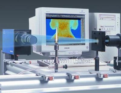

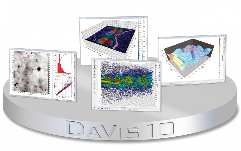
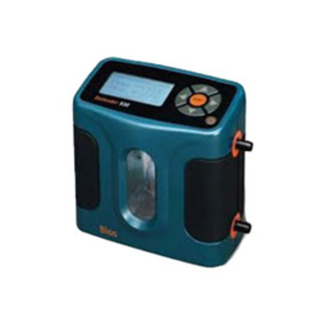


 咨询
咨询