脑动脉瘤模型中体外体视粒子成像测速检测方案(CCD相机)

智能文字提取功能测试中

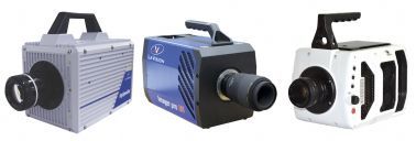
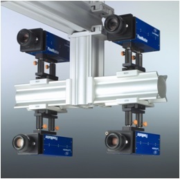
(a) Patient-Specific Cerebral Aneurysm Hemodynamics：Comparison of in vitro Volumetric Particle Velocimetry，Computational Fluid Dynamics (CFD)， and in vivo 4D FlowMRI Melissa C. Brindisel， Sean Rothenberger²， Benjamin Dickerhoff’， Susanne Schnell， Michael Markl4，5，David Saloner， Vitaliy L.Rayz?， Pavlos P. Vlachos 1School of Mechanical Engineering， Purdue University， West Lafayette， IN 2Weldon School of Biomedical Engineering， Purdue University， West Lafayette， IN 3Department of Biomedical Engineering， Marquette University， Milwaukee， WI 4Feinberg School of Medicine， Northwestern University， Chicago， IL McCormick School of Engineering， Northwestern University， Evanston， IL Department of Radiology and Biomedical Imaging， University of California San Francisco， CA Corresponding Author： Pavlos P. Vlachos Email： pvlachos@purdue.edu Address： 585 Purdue Mall， West Lafayette， IN， 47907 Abstract Typical approaches to patient-specific hemodynamic studies of cerebral aneurysms use image based computationalfluid dynamics (CFD) and seek to statistically correlate parameters such as wall shear stress (WSS) and oscillatoryshear index (OSI) to risk of growth and rupture. However， such studies have reported contradictory results，emphasizingthe need for in-depth comparisons of volumetric experiments and CFD. In this work， we conducted tomographic particlevelocimetry experiments using two patient-specific cerebral aneurysm models (basilar tip and internal carotid artery)under pulsatile flow conditions and processed the particle images using Shake the Box (STB)， a particle tracking method.The STB data was compared to that obtained from in vivo 4D flow MRl and CFD. Although qualitative agreement of flowpathlines across modalities was observed， each modality maintained notably unique spatiotemporal distributions of lownormalized WSS regions. Analysis of time averaged WSS (TAWSS)， OSI， and Relative Residence Time (RRT)demonstrated that non-dimensional parameters， such as OSI， may be more robust to the varying assumptions，limitations， and spatial resolutions of each subject and modality. These results suggest a need for further multi-modalityanalysis as well as development of non-dimensional hemodynamic parameters and correlation of such metrics toaneurysm risk of growth and rupture. Keywords： Cerebral aneurysm，particle velocimetry， 4D Flow MRI， computational fluid dynamics， wall shearstress， oscillatory shear index 1 Introduction It is estimated that about 3% of the population harbors an unruptured intracranial aneurysm(IA)[1]. If detected， clinicians must assess and balance risk of rupture with risk of treatment of thecerebral aneurysm [2，3]. However， accurately assessing risk of rupture in IAs is difficult as thespecific mechanisms that cause an aneurysm to form， grow， and rupture remain largely unknown. Previous studies have demonstrated that hemodynamics play a critical role in the growth andrupture of an IA [4-8]. However， despite a large volume of studies that have investigated theinfluence of several hemodynamic variables on risk of rupture， contradictory and ultimatelyinconclusive results have been reported. Wall shear stress (WSS) has received much attention， buthas been perhaps the most controversial hemodynamic parameter [8]. Both low [4，9-12] and high[13，14] WSS have been shown to indicate elevated risk of rupture. High WSS gradients， highoscillatory shear index (OSI)， and high relative residence time (RRT) have also been reported toincrease risk of rupture [4，8，11，15]. Studies have also explored the presence and effect of chaoticflow and high frequency fluctuations in cerebral aneurysms [3，6，16]. Other hemodynamic variablesidentified as potentially increasing risk of rupture include concentrated inflow jets， larger shearconcentration， lower viscous dissipation， and complex and unstable flow patterns[6，13，14]. Computational fluid dynamics (CFD) has been the predominant methodology used to studyhemodynamics in cerebral aneurysms [2，4，9，10，14，16]. However， limited CFD validation anddisputed CFD assumptions such as laminar flow remain issues limiting its clinical acceptance [17].It has also been shown that CFD results can vary significantly based on solver parameters， evenwhen similar geometries and boundary conditions are used [5]. Velocity fields obtained from both invivo and in vitro 4D Flow MRI have also been used， but the low spatiotemporal resolution is a majorlimitation of this modality [5，10，18]. Although high resolution 4D Flow MRI has been shown tocapture complex flow patterns [18]， studies have demonstrated that the low resolution causes anunderestimation of velocity and WSS magnitudes， particularly when compared to CFD or PIV[2，5，10，19]. Few experimental particle image velocimetry (PIV) studies have been conducted in thisdomain. Among such studies， planar and stereo PIV (2D-2 velocity component) have been mostcommon [3，11，15，18，20]. Other studies have taken 2D data at several parallel planes in a"slicedplanar”(3D-2 velocity component) configuration and subsequently reconstructed the third velocitycomponent [6，21]. Despite the high three-dimensionality known to exist in cerebral aneurysmgeometries， to date， only one steady flow 4D volumetric PIV (3D-3 velocity component) study hasbeen reported [5]. Further， PIV studies are most often used only to compare flow patterns andvalidate CFD models and simulations [5，11，18]，only a few have reported WSS and even less OSIand RRT [6，15]. In this work， we conducted one of the first reported pulsatile volumetric particle velocimetrystudies using two patient-specific aneurysm models. As opposed to traditional PIV studies whichuse interrogation window correlation， we used Shake the Boxx (STB)， a particle trackingmethodology， which has， to the authors'knowledge， never been used in this domain. We comparethe STB results with those obtained using both CFD and in vivo 4D Flow MRl. All three modalitiesmaintain different assumptions and limitations that can affect subsequent hemodynamic analysis.In this work， we investigate the effect of spatial resolution and modality on time averaged WSS(TAWSS)， OSI， and RRT. 2 Materials and Methods 2.1 In vivo 4D Flow MRl and MRA imaging Table 1： 4D Flow MRI parameters and resolutions Geometry TE/TR Flip Velocity Encoding Temporal Spatial Resolution (ms) Angle() (venc) (cm/s) Resolution (ms) (mm) Basilar Tip 3.46/6.33 12 100 40.5 1.25x1.25x 1.33 ICA 2.997/6.4 15 80 44.8 1.09 x 1.09x1.30 The two aneurysm models used were a basilar tip aneurysm， MRI imaged at the SanFrancisco VA Medical Center， and an internal carotid artery (ICA) aneurysm， MRl imaged atNorthwestern Memorial Hospital (NMH). Both aneurysms were imaged on a 3T MRI scanner (Skyra，Siemens Healthcare， Erlangen， Germany). At San Francisco VA Medical Center， the Siemens WIPsequence， an ECG-gated RF spoiled 4D Flow MRI sequence was used with gadolinium contrast，while at NMH no contrast was used. The 4D flow scan parameters for both imaging studies aregiven in Table 1. The in vivo 4D Flow MRI data will be referred to simply as ‘4D Flow'herein. All 4D Flow data was corrected for noise， velocity aliasing， and phase offset errors causedby eddy currents and concomitant gradient terms. In addition to 4D Flow， contrast-enhancedmagnetic resonance angiography (CE-MRA) data with a spatial resolution of 0.7 x0.7 x0.7 mmforthe basilar tip aneurysm and non-contrast time of flight (TOF) angiography with a spatial resolutionof 0.4x0.4 x0.6 mmfor the ICA aneurysm were acquired in the same scanning sessions and usedto create the in vitro models. 2.2 Image segmentation and model fabrication For the basilar tip aneurysm， CE-MRA images were segmented using an in-house VTK-based software. A 3D iso-surface was computed by selecting a threshold intensity value that definedthe intra-luminal volume of the vessel. The threshold was adjusted to match the iso-surface to the MR luminal boundaries. For the ICA aneurysm，TOF images were segmented with open-sourcelTK-SNAP software， using thresholding andvolume growth techniques. A modeling software，Geomagic Design (3D Systems， Rock Hill， SC)，was used to separate the inflow and outflowvessels of the aneurysm from the remainingcerebral vasculature (Figures 1a and 1c). Theresulting surface (STL)， shown in Figures 1b and1d， was used for CFD simulations and flowphantom fabrication. For the flow phantoms， inletand outlet vessels were extended in order toconnect the model to the flow loop. A positive-space model of the vascular geometry was 3Dprinted (ProJet printer - 3D Systems)， embeddedinto a tear-resistant silicone block， then cut fromthe block. A low melting point metal (Cerrobend158 Bismuth alloy) was cast into the block and (a) (b)12- the block was then cut away. The metal model Figure 1： Segmentation from (a) in vivo vasculature showingpatient-specific basilar tip aneurysm， to the (b) associated in vitromodel. (c) In vivo vasculature for patient-specific internal carotidartery (ICA) aneurysm and the (d) in vitro segmented model.(PCA=posterior cerebral artery， SCA=superior cerebellar artery，MCA=middle cerebral artery， ACA=anterior cerebral artery，PComA= posterior communicating artery). was embedded in optically clear polydimethylsiloxane silicone (PDMS-Slygard 184) which wasallowed to cure until hardened， then the metal was melted out from the clear PDMS. 2.3 In vitro flow loop An in vitro flow loop (Figure 2a) was designed to simulate in vivo flow conditions. The workingfluids， detailed in Table 2， were blood analogs consisting of water， glycerol， and urea [22]. Thepulsatile inflow waveforms (Figure 2b) were extracted from the in vivo 4D Flow MRI data andgenerated by a computer-controlled gear pump. Average flow rates for the outlet vessels werecontrolled using resistive elements to match the 4D Flow outlet flow rate ratios. Flow details for bothgeometries are provided in Table 3. Table 2： Blood analog working fluids used for both geometries.Nano-pure water， technical grade glycerol (99%-McMaster-Carr)， and99+% urea (Fischer Scientific) were used. Geometry Blood Analog Composition (%wt) Density (kg/m) Kinematic Water Glycerol Urea Viscosity (m²/s) Basilar Tip 44.8 32.8 22.4 1103 3.04x10 ICA 45.3 29.7 25.0 1132 3.50x10- Table 3： Flow cycle information for both aneurysm geometries Geometry Reynolds Number Womersley Cycle Period，T Max Min Number (seC) Basilar Tip 500 150 2.73 0.77 ICA 300 130 5.33 0.54 Figure 2： (a) Schematic of the flow loop setup， including the camera and calibration plate setup. F indicates locations of ultrasonicflowmeters and P indicates locations of pressure transducers.(b) Inflow flow rate and pressure taken from the upstream flow meter andpressure transducers for both geometries. The phase of the pulsatile cycle is displayed as it was extracted from 4D Flow MRI. (c)Sample Shake the Box tracks for the ICA geometry. 2.4 Volumetric particle velocimetry measurement technique Particle images were captured using an Nd-YLF laser (Continuum Terra-PIV， A = 527 nm)and four high-speed cameras (Phantom Miro). In the camera configuration (Figure 2a)，the centercamera was not angled， while the other three were angled about 30°from the geometry plane. Themagnification of all cameras was approximately 30 um/pixel. Flow was seeded with 24 pmfluorescent particles and long-pass filters filtered the laser light from the images. The index of refraction of the working fluid was matched to that of the PDMS model (n=1.4118)， and the modelwas submerged in the working fluid to reduce optical distortion. Time-resolved images (1216x1224pixels for basilar tip， 1088x1320 pixels for ICA) were captured at 2000 Hz， corresponding to amaximum particle displacement between frames of approximately 10 pixels. Three full pulsatilecycles for the basilar tip aneurysm and four cycles for the ICA aneurysm were captured. Particle images were processed using DaVis 10.0 (LaVision Inc.). Calibration images werecaptured using a dual-plane calibration target. The perspective calibration error was approximately0.25 pix for each camera in both experiments and volume self-calibration corrected these errors toless than 0.03 pix [23]. Rather than using 3D volume correlation as used in tomographic PIV， Shakethe Box (STB)， a particle tracking based algorithm， was used to process the velocity fields. SampleSTB tracks are shown in Figure 2c. STB reduced the prevalence of ghost particles (falselytriangulated 3D particles)， which are expected to be high in these complex geometries and can create significant bias error [24，25]. STB requires time-resolved data， using the previous timestep to iteratively add predicted particle locations in the next time step. The predicted particlelocations are refined by iteratively “shaking" them within a tolerance， minimizing the residualbetween the subsequent particle image and predicted particle image. The STB was done using 12iterations for both the outer (adding particles) and inner (particle position refinement) loops with anallowed particle triangulation error of 1.5 voxels and particle position shaking of 0.1 voxels. Currently，no methods to evaluate uncertainty using STB processing have been reported， however， thecalibration errors were consistent with those observed in well-controlled tomographic PIVexperiments. The volumetric STB data will be referred to as ‘STB'herein. 2.5 CFD simulation CFD simulations were performed using Fluent 18.1 (ANSYS) to solve the governing Navier-Stokes equations. An unstructured tetrahedral mesh was generated on the domain usingHyperMesh 14.0 (Altair Engineering， Troy，MI). Incompressible，Newtonian flow with density of 1060kg/m’and dynamic viscosity of 0.0035 Pa's was modeled. Laminar flow and rigid walls wereassumed. Patient-specific waveforms obtained from 4D Flow were prescribed at the inlet and outletsof the CFD models. A pressure-based coupled algorithm was used to solve the momentum andpressure-based continuity equations. A second-order Crank-Nicolson scheme was used in timediscretization and a third-order MUSCL scheme was used for discretization of the momentumequations. A mesh with the nominal cell size of 150 pm and time step of 1.5 ms was used. Thesevalues provided sufficient resolution of the flow based on mesh independence and temporalresolution testing. Three cardiac cycles were simulated， and the results obtained for the last cyclewere used for comparisons with the other modalities. 2.6 Post-processing All modalities were registered to and masked by the STL geometry obtained from MRAsegmentation. The unstructured STB and CFD data were gridded to isotropic resolutions of 0.3 and0.4 mm for the basilar tip and ICA aneurysms， respectively， using inverse-squared radial distanceweighted averaging. An initial radius of half the grid size was used to search for the nearestunstructured vectors， however this radius was extended to ensure a minimum of three unstructuredvectors for each averaging calculation. For the STB gridding， unstructured velocity fields weretemporally grouped at a 5：1 and 3：1 ratio for the basilar tip and ICA aneurysms， respectively， suchthat each unstructured field was used in only a single group. This increased the number ofunstructured particles per gridded time step but reduced the effective temporal resolution to 2.5 ms and 1.5 ms for the basilar tip and ICA aneurysms， respectively. The gridded STB data was filteredusing proper orthogonal decomposition (POD) with the entropy line fit (ELF) autonomousthresholding method [26，27]. A single pass of universal outlier detection (UOD) [28] and phaseaveraging of the STB pulsatile cycles were subsequently done.“Virtual voxel averaging”wasspatially performed to bring the STB and CFD data to the 4D Flow spatial resolution. Wall shear stress was computed using thin-plate spline radial basis functions (TPS-RBF)，which performs smoothing surface fits and reduces errors in the inherently noisy gradient calculation[29]. A normal vector at each surface point was computed by mapping the velocity coordinate to theequivalent STL-surface point and computing the inward facing normal from a surface fit of 25adjacent STL-surface points. Two passes of UOD were used to eliminate erroneous normal vectors.For the voxel averaged datasets， wall normals were extracted from their full resolution equivalent.For the 4D Flow， the full resolution CFD was used.WSS was computed according to the followingequations [30]： where Tx， Ty， and tz， are the WSS components in the x，y， and z directions， Tmag is the WSSmagnitude， u is the dynamic viscosity，and (nx， ny， nz) is the unit normal. The in-house WSS code， including the wall normal and velocity gradient calculations， wasvalidated using analytical 3D Poiseuille flow data. Biases in the near-wall discrete velocity gradients，whose magnitude vary based on each specific point’s distance from the wall， is a known issue [6，29].Thus， similar to that done in Yagi et al. (2013) [6]， the WSS calculation was extended to usegradients beyond the biased near-wall region， mitigating the spatial variation of this bias to about5% but allowing WSS magnitude bias errors of up to 25% (based on the validation testing). Thus，allWSS magnitudes reported here are expected to have a consistent bias and should be consideredonly relative to other values reported here. Time averaged WSS (TAWSS) was computed according to Eq. 2.5 where tw is the WSS vector and T is the duration of the pulsatile cycle. Oscillatory shear index (OSI)was subsequently computed according to Eq.2.6 OSl is a non-dimensional parameter ranging from 0 to 0.5， where 0 indicates no oscillatory WSSthroughout the pulsatile cycle and 0.5 indicates oscillatory WSS throughout the entire pulsatile cycle.Relative residence time (RRT) was computed using Eq. 2.7 3 Results 3.1 Comparing flow structures and WSS across modalities The inlet flow rate computed from the velocity fields for all modalities in the basilar tip and Figure 3： Inlet flow rates for all modalities in the (a) basilar tipaneurysm and (b) ICA aneurysm.3 ICA\ianeurysmss were computed to ensureagreement across modalities and are shown inFigures 3a and 3b， respectively. Because of thelow spatial resolution of 4D Flow， a largeruncertainty of the computed flow rate wasexpected. The maximum inlet flow rate in thebasilar tip aneurysm was 4.28， 4.89， and 5.61mL/s for the 4D Flow and full resolution STB andCFD， respectively. The average inlet flow ratewas 2.58 mL/s for the 4D Flow， 3.48 mL/s forSTB， and 3.51 mL/s for CFD. The trend of the inflow waveforms was similar for all modalities， with STB maintaining the largest temporal variabilityamong modalities as expected. For the ICA aneurysm， the maximum inflow rate was similar for allmodalities at 5.46， 5.40， and 5.26 mL/s for the 4D Flow， and full resolution STB and CFD，respectively.The average inlet flow rate was 4.26 mL/s for 4D Flow， 4.00 mL/s for STB， and 3.79mL/s for CFD. Again， good agreement of the inflow waveform trend was observed across allmodalities. Figure 4 shows the 3D velocity pathlines for each modality and geometry at peak systole.Initial observation shows qualitative agreement of the flow patterns across all modalities for bothgeometries. In the basilar tip aneurysm (Figure 4a) flow enters from the basilar artery and about20% exits through the superior cerebellar arteries (SCAs). The remainder of the flow extends intothe right distal posterior region of the aneurysmal sac， swirls to the left proximal anterior portion ofthe sac and exits the posterior cerebral arteries (PCAs). In the ICA aneurysm (Figure 4b) flow entersfrom the curving ICA and some flow rotates through the aneurysmal sac before re-entering the distalICA. About half of the flow exits through the middle cerebral artery (MCA) and the remainder splitsbetween the anterior cerebral artery (ACA) and posterior communicating artery (PComA). Theswirling flow in the aneurysmal sac was qualitatively similar for the 4D Flow and CFD， while for theSTB the swirling was more centered in the sac. Figure 5 illustrates the WSS distribution at peak systole， normalized by the maximum peaksystole WSS for each modality. The same WSS calculation method was used for all modalities. Forboth geometries， despite the similarities in the flow rate and flow structure， significant spatial Figure 4： Velocity field pathlines for the MRI and full resolution STB and CFD at peak systole for the (a) basilar tip aneurysm and(b)ICA aneurysm. (Note： The two aneurysm geometries (a) and (b)are not shown at the same spatial scale.) 4D Flow—STB-Full—CFD-Full wall shear stress (dynes/cm) Figure 5： Normalized wall shear stress distribution for all modalities in the (a) basilar tip aneurysm and (b) ICA aneurysm. (Note： Thetwo aneurysm geometries (a) and (b) are not shown at the same spatial scale.) The PDF of wall shear stress in the aneurysmal sac for allmodalities and resolutions in the (c) basilar tip aneurysm and (d) ICA aneurysm. differences among the WSS across all modalities were observed. For the basilar tip aneurysm(Figure 5a)， the full resolution CFD exhibited a large region of low WSS at the proximal anteriorportion of the aneurysmal sac. Conversely， the full resolution STB showed no region of low WSSand 4D Flow maintained a much smaller region of low WSS at that location. For the ICA aneurysm(Figure 5b)， 4D Flow， STB， and CFD all indicated uniquely different regions of low WSS. In this case，STB indicated the entire aneurysmal sac having low WSS， while CFD results showed patches oflow WSS at the anterior and posterior faces of the aneurysmal sac， and 4D Flow showed nosignificant low WSS regions. Except for the STB results in ICA aneurysm， no regions of low WSSamong the voxel averaged datasets were observed. In terms of WSS magnitude， for the basilar tipaneurysm (Figure 5c)， the full resolution STB and CFD had similar PDF distributions， with STBmaintaining slightly higher magnitudes. 4D Flow had slightly lower WSS magnitude than thatobtained in STB and CFD. The voxel averaged STB and CFD maintained similar distributions ofWSS magnitude. For the ICA aneurysm (Figure 5d)， the WSS magnitude distributions of the 4DFlow and full resolution STB matched well. The voxel averaged STB and CFD distributions also hadsimilar distributions to that of the 4D Flow， with slight under and over estimations comparatively.Conversely， the full resolution CFD WSS distribution maintained a larger spread of WSS values thanall other modalities and maintained the largest WSS magnitudes. 3.2 Effect of modality and spatial resolution on TAWSS， OSI， and RRT The previous section’s results suggested that WSS is highly sensitive to the methods，assumptions and limitations associated with different modalities， even when flow rates and flowstructures showed good agreement. To further explore this notion， the influence of the differentmodalities and effect of spatial resolution on TAWSS， OSl， and RRT was evaluated. Figure 6 shows the distributions of TAWSS， OSI， and RRT in the aneurysmal sac for allmodalities for the basilar tip aneurysm (Fig 6a-c) and ICA aneurysm (Fig 6d-f). The interquartileranges and 95% confidence intervals are also provided. In agreement with the previous results， thedistributions of the TAWSS varied significantly across all five data sets. In the basilar tip aneurysm，the average TAWSS was 9.21 dynes/cm² for the 4D Flow， 16.14 dynes/cm for the full resolutionSTB， and 11.61 dynes/cm² for the full resolution CFD. When voxel averaged， the average TAWSS 40 (a) (d) Figure 6：Distribution of (a) timeaveraged wall shear stress(TAWSS)， (b) oscillatory shearindex (OSI)，and (c) relativeresidence time (RRT) in thebasilar tip aneurysm， where widthof PDF shows relative distributiondensity. Distribution of (d)TAWSS，(e) OSI， and (f) RRT inthe ICA aneurysm. Mean andmedian values， interquartileranges， and 95% confidenceintervals are indicated. 4D Flow STB-VA STBCFD-VAACFD 4D Flow STB-VA STBBCFD-VA CFD PDF—Mean -MedianIQR—95% Cl decreased to 7.39 dynes/cm² for the STB， a 54% drop， and to 6.82 dynes/cm² for the CFD， a 41%decrease. For the ICA aneurysm， the average TAWSS for STB had only a small change from 2.28to 2.06 dynes/cm2 when voxel averaged. The average CFD TAWSS decreased 70% from 8.25 to2.46 dynes/cm² when voxel averaged. The average OSI of the STB for the basilar tip aneurysmchanged from 0.12 to 0.11， while CFD went from 0.04 to 0.07 when voxel averaged. Voxel averagingchanged the average OSl in the ICA aneurysm from 0.16 to 0.09 for STB and from 0.06 to 0.08 forCFD. In terms of RRT， the average RRT was 0.47， 0.28， and 0.29 (dynes/cm2)-1 for the 4D Flow，and full resolution STB and CFD， respectively， in the basilar tip aneurysm. When voxel averaged，these values changed to 1.22 (dynes/cm2)-1 for STB and 0.50 (dynes/cm2)-1 for CFD. Average RRTin the ICA aneurysm was 1.93， 1.38， and 0.42 (dynes/cm2)-1 for the 4D Flow， and full resolution STBand CFD，respectively. Voxel averaging increased the average RRT to 2.62 (dynes/cm2)-1 for STBand to 1.27 (dynes/cm2)1 for CFD. Overall， the median OSI change was about 40% when data wasvoxel averaged while the median TAWSS and RRT changes were 48 and 145%， respectively. To investigate the effect of spatial resolution on TAWSS， OSI， and RRT in more detail， Figure7 illustrates Bland-Altman analysis comparing the voxel averaged and full resolution STB and CFDacross the entire flow domain. In both aneurysms， a proportional error of the TAWSS was observedwhere the voxel averaged TAWSS magnitude was less than that of the full resolution， in agreementwith the results in Figure 6. The average differences were -10.52 and -6.02 dynes/cm² for the STBand CFD， respectively， in the basilar tip aneurysm (Fig 7a). For the ICA aneurysm (Fig 7b)， theaverage TAWSS difference was -0.16 dynes/cm² for STB and -8.70 dynes/cm² for CFD. Theaverage OSI difference magnitude across all cases was 0.02， with a maximum difference magnitudeof 0.05. The spread of OSI points was relatively symmetric， demonstrating no significant bias orproportional error. In the basilar tip aneurysm， the average RRT difference was 0.77 (dynes/cm2)-1 Data Points· 95%CI——Mean Diff Figure 7： Bland-Altman analysis of time averaged wall shear stress， oscillatory shear index， and relative residence time， comparingvoxel averaged STB to full resolution STB and voxel averaged CFD to full resolution CFD in the (a) basilar tip aneurysm and(b)ICA aneurysm. Mean difference and 95% confidence intervals are indicated. for the STB and 0.35 (dynes/cm2)-1 for the CFD， and 2.27 and 0.51 (dynes/cm2)-1 for the STB andCFD， respectively， in the ICA aneurysm. A similar proportional type error was observed with theRRT as with the TAWSS， but in this case the voxel averaged RRT was larger in magnitude thanthat of the full resolution. Thus， Figure 7 confirms the varying behavior and sensitivity of each metricto spatial resolution. With the different behavior of the TAWSS， OSI， and RRT metrics， it is of interest to determinehow the metrics perform when comparing the in vitro and in silico data to the in vivo 4D Flow dataas well as how the spatial resolution of the in vitro and in silico datasets affect the comparison.Thus，Bland-Altman analysis was performed to compare these metrics in the aneurysmal sac computedfrom 4D Flow to those computed from other modalities (Figure 8). In the basilar tip aneurysm (Fig8a)， the mean TAWSS difference was -7.45 and -2.1 dynes/cm² for the full resolution STB and CFD，respectively. This changed to 1.72 dynes/cm² for the voxel averaged STB and 2.52 dynes/cm forthe voxel averaged CFD. The 95% confidence intervals for the voxel averaged data reduced inrange by 44% for STB and 31% for CFD as compared to the full resolution intervals. Similar trendswere observed in the ICA aneurysm TAWSS (Fig 8b). The mean difference was -0.63 dynes/cm²for the full resolution STB and -8.92 dynes/cm for the full resolution CFD. The 95% confidence · Data Points -95% Cl—Mean Diff Figure 8： Bland-Altman analysis of time averaged wall shear stress， oscillatory shear index， and relative residence time， comparing invivo 4D Flow MRI to voxel averaged STB (STB-VA)， full resolution STB， voxel averaged CFD (CFD-VA)， and full resolution CFD in the(a) basilar tip aneurysm and (b) ICA aneurysm. Mean difference and 95% confidence intervals are indicated. interval limits reduced by 51 and 70% for the voxel averaged STB and CFD， respectively， ascompared to the full resolution data. Thus， the voxel averaged datasets generally maintained abetter match to the 4D Flow TAWSS than the full resolution datasets. In terms of OSI， the meandifference was -0.02 and 0.05 for the full resolution STB and CFD， respectively， in the basilar tipaneurysm. Voxel averaging had a minimal effect， changing the mean difference to 0.01 for CFD andcausing no change in STB. Further， the 95% confidence intervals reduced by only 18% for STB and9% for CFD when voxel averaged. Mean OSI differences of 0.01 for the full resolution STB， 0.07 forthe voxel averaged STB， 0.13 for the full resolution CFD， and 0.09 for the voxel averaged CFD wereobserved in the ICA aneurysm. The interval ranges decreased by 18% when voxel averaged for theSTB and increased by 16% when voxel averaged for the CFD. In the basilar tipaneurysm， the meanRRT difference was 0.22 and-0.83 (dynes/cm2)-1 for the full resolution and voxel averaged STB，respectively， and 0.18， and -0.02 (dynes/cm2)1 for the full resolution and voxel averaged CFD，respectively. The confidence interval ranges increased 10-fold for the STB when voxel averagedand 3-fold for the CFD when voxel averaged. For the ICA aneurysm， the mean RRT difference was0.34 (dynes/cm2)-1 for the full resolution STB and -0.87 (dynes/cm2)-1 for the voxel averaged STB.The mean RRT difference was 1.60 and 0.49 (dynes/cm2)-1 for the full resolution and voxel averagedCFD， respectively. The confidence intervals maintained about 4-fold increases in range for the voxelaveraged CFD datasets as compared to the full resolution datasets. The RRT confidence intervalranges suggests a better match between the in vivo4D Flow and full resolution datasets， thoughthe mean differences were similar between full and voxel averaged resolutions. 4 Discussion The goal of this work was to compare in vivo 4D Flow MRI， in vitro experimental particlevelocimetry， and CFD using two patient-specific cerebral aneurysm models in order to investigatehow the limitations， assumptions， and spatial resolutions unique to each modality affectedhemodynamic metrics including TAWSS， OSI， and RRT. Experimental PIV studies are significantlyless common in this domain than CFD studies， and OSI and RRT have rarely， if ever， been computed using experimental PIV data. However， because experimental studies produce measuredrather than simulated velocity fields and typically require less assumptions on the flow， when wellcontrolled， they can often provide a higher fidelity representation of the flow. The use of all threemodalities rather than any one or two provided a richer span of the assumptions and limitations thatcan affect hemodynamic metrics， demonstrating a need for additional comparison studies usingvolumetric particle velocimetry in this domain. In general， the results of this study demonstrated thelimitations and assumptions associated with each modality can have significant effects onhemodynamic metrics. Analysis of TAWSS， OSI， and RRT demonstrated that OSI， a non-dimensional parameter， was most robust to changing modalities (and thus assumptions) and spatialresolutions. Low WSS regions and their impact on risk of rupture have received much attention in thisdomain [4，8-11，15]. As seen in Figure 5， all modalities had uniquely different regions of low WSSin the aneurysmal sacs of both geometries， despite the general qualitative agreement of inflowwaveforms and velocity pathlines. In this study， WSS was computed using the same methodology，hence the variation cannot be attributed to different calculation biases. Further， Cebral et al. (2011)[14] showed inflow waveform changes can cause variability on the magnitude， but not spatialvariation， of hemodynamic metrics. Thus， because the normalized coherent regions of low WSS areof interest， the WSS difference cannot be attributed to variations in inflow rate across modalities.Therefore， this WSS difference was most likely attributable to differences in the assumptions andlimitations of each modality. For example， segmentation uncertainties among the in vitro and in silicodata sets， the laminar flow assumptions used in CFD simulations， and the curved extension of theinflow vessel required for experimental model manufacturing for the STB data all could have affectedthe WSS spatial distributions to some extent. Such assumptions had only small effects on thevelocity field and flow patterns but， as shown here， maintained greater variation on the WSSdistribution. Thus， the WSS uncertainty resulting from each assumption for each modality must becarefully considered and explicitly studied in future work. Overall， this difference in WSS distributioncarries significant clinical and research implications. With the link of low WSS regions to thelocations of aneurysm rupture [9，15]， the predicted stability of the aneurysm would be differentbased on the WSS distribution obtained from full resolution CFD versus that obtained from fullresolution STB， particularly for the basilar tip aneurysm. Further， studies which investigatehemodynamic variables and analyze which variables have a statistically significant differencebetween ruptured and unruptured aneurysms， regardless of modality， rely on various flowassumptions which could be largely altering WSS distributions， thus confounding statisticallysignificant results. The effect of spatial resolution on both velocity and wall shear stress magnitude has been agrowing concern. Roloff et al.(2018)[5] demonstrated reductions of velocity magnitude by as muchas 10-20% because of voxel averaging. van Ooij et al. (2013)[10] reported WSS values for 4D FlowMRI were lower than that of CFD，but increased if the MRI spatial resolution was increased. Figure8 agrees with this notion， demonstrating that datasets with similar spatial resolutions have similarTAWSS magnitudes. Specifically， lowering the spatial resolution generally lowers the wall shearstress magnitude. In Figure 7， reduction (bias error) of TAWSS caused by virtual voxel averagingwithin the same modality was about 6.35 dynes/cm2， corresponding to a roughly 81% error whennormalizing by the mean TAWSS across all datasets. Similarly， the average RRT error caused byvoxel averaging was 0.98 (dynes/cm2)1， a 91% error when normalizing by the mean RRT across alldatasets. However， the average OSI bias error caused by voxel averaging was 0.02， a 26% errorwhen normalized by the mean OSI across all datasets. Further， in Figure 8， when comparing the invitro and in silico datasets to the in vivo 4D Flow， OSI not only maintained the lowest bias errors (relative to the mean values)， but also the most consistent 95% interval bounds across all modalitiesas well as across full resolution and voxel averaged datasets within the same modality. Thus， OSIwas more robust to modality and spatial resolution， and maintained more consistent results thanboth TAWSS and RRT. OSI yielded no proportional or significant bias errors for all datasets andcomparisons. Because OSl is a non-dimensional parameter， its magnitude is less affected by biaserror than equivalent dimensional parameters， as bias scale errors in the WSS magnitude wouldcancel out in the OSI calculation (Equation 2.6). Bias errors are unavoidable across all modalitiesand subjects and are attributed， at least in part， to the assumptions and spatial resolution of the dataas well as calculation methodologies. Thus， OSI and other non-dimensional parameters offer thepotential for more consistent risk analysis metrics across a cohort of varying geometries and 4DFlow resolutions than equivalent dimensional parameters. This is a notion that should be exploredand expanded in future studies. There were several limitations of this study. The inlet vessel of the in vitro models had to becurved slightly for experimental and manufacturing reasons. This could have had some effect oninflow conditions of the STB experiment， possibly preventing fully developed inflow. Although notideal， given the natural tortuosity of the cerebral vasculature， the exact in vivo inflow conditionswould be complex and therefore could not be matched regardless. Further， the resistance valvesused to control the outlet flow rates could only adjust the average flow rate in the vessel and not thepulsatility of the flow rate. Thus， some differences in the flow rate range of smaller vessels wasobserved. Uncertainty quantification methods are widely available for PlV but have yet to bereported for STB and are needed so this data can be used as robust validation test cases for CFDsimulations. While virtual voxel averaging was done here， this process does not exactly replicatethat of MRI voxel or ensemble averaging. Thus， additional studies are needed to further explore thepossible effects of voxel averaging on velocity and post-processing metrics identified in this studyusing higher fidelity voxel averaging techniques. Bias errors in discrete WSS calculations are welldocumented in the literature [6，29]. From the WSS algorithm validation done for this study， aconsistent bias error was a known issue. Therefore， all WSS， OSI， and RRT values reported in thisstudy can validly be interpreted in a relative sense， but global values of these metrics cannot beextrapolated from this study. 5 Conclusion The goal of this study was to compare in vitro volumetric flow velocimetry data with CFD andin vivo 4D Flow MRl in order to investigate how the modality and spatial resolution affect TAWSS，OSI， and RRT. The similarity of flow patterns but notable differences in low WSS distributions acrossmodalities demonstrated that more in-depth and comprehensive analysis of specific modelingassumptions and their effect on hemodynamic parameters is needed. Further， non-dimensionalparameters， such as OSI， were shown to be more robust and consistent to varying spatialresolutions and modalities， a finding which can improve flow metrics associated with aneurysm riskof rupture in future work. However， given the limitations of this study， additional studies andcomparisons are needed to further investigate these findings. 6 Acknowledgements American Heart Association pre-doctoral fellowship (17PRE33670268) to Melissa Brindise， and NIHawards R21 NS106696 and R01 HL115267 (V. Rayz) are gratefully acknowledged. 7 Conflict of interest The authors have no conflicts of interest to report. 8 Human and Animal Rights Patient consent was not required. No human or animal studies were carried out by the authors forthis article. 9References 1. Vlak MHM， Algra A， Brandenburg R， Rinkel GJE. Prevalence of unruptured intracranialaneurysms， with emphasis on sex， age，comorbidity， country， and time period： A systematicreview and meta-analysis. Lancet Neurol.2011；10(7)：626-36. 2. Rayz VL， Abla A， Boussel L， Leach JR， Acevedo-Bolton G， Saloner D， et al. ComputationalModeling of Flow-Altering Surgeries in Basilar Aneurysms. Ann Biomed Eng.2015；43(5)：1210-22. 3. Ford MD， Nikolov HN， Milner JS， Lownie SP， Demont EM， Kalata W， et al. PIV-measuredversus CFD-predicted flow dynamics in anatomically realistic cerebral aneurysm models. JBiomech Eng. 2008 Apr；130(2)：021015. 4. Xiang J， Natarajan SK， Tremmel M， Ma D， Mocco J， Hopkins LN， et al. Hemodynamic-morphologic discriminants for intracranial aneurysm rupture. Stroke. 2011；42(1)：144-52. 5. Roloff C， Stucht D， Beuing O， Berg P. Comparison of intracranial aneurysm flowquantification techniques： standard PlV vs stereoscopic PIV vs tomographic PIV vs phase-contrast MRI vs CFD. J Neurointerv Surg. 2018；neurintsurg-2018-013921. 6. Yagi T， Sato A， Shinke M， Takahashi S， Tobe Y， Takao H， et al. Experimental insights intoflow impingement in cerebral aneurysm by stereoscopic particle image velocimetry：transition from a laminar regime. J R Soc Interface. 2013；10(82)：20121031. 7. Cebral JR， Raschi M. Suggested connections between risk factors of intracranialaneurysms： A review. Ann Biomed Eng. 2013；41(7)：1366-83. 8. Meng H， Tutino VM，Xiang J， Siddiqui A. High WSS or Low WSS? Complex interactions ofhemodynamics with intracranial aneurysm initiation， growth，and rupture： Toward a unifyinghypothesis. Am J Neuroradiol. 2014；35(7)：1254-62. 9. Boussel L， Rayz V， McCulloch C， Martin A， Acevedo-Bolton G， Lawton M， et al. Aneurysmgrowth occurs at region of low wall shear stress： Patient-specific correlation ofhemodynamics and growth in a longitudinal study. Stroke. 2008；39(11)：2997-3002. 10. van Ooij P， Potters WV.， Guedon A， Schneiders JJ， Marquering HA， Majoie CB， et al. Wallshear stress estimated with phase contrast MRI in an in vitro and in vivo intracranialaneurysm. J Magn Reson Imaging. 2013；38(4)：876-84. 11. Kojima M， Irie K， Ikeda S， Fukada T， Arai F， Hirose Y， et al. The hemodynamic study forgrowth factor evaluation of rupture cerebral aneurysm followed up for five years. J BiomedSci Eng. 2012；05(12)：884-91. 12. Xu j， Yu Y， Wu X， Wu Y， Jiang C， Wang S， et al. Morphological and Hemodynamic Analysisof Mirror Posterior Communicating Artery Aneurysms. PLoS One. 2013；8(1)：1-7. 13. Castro MA， Putman CM， Sheridan MJ， Cebral JR. Hemodynamic patterns of anteriorcommunicating artery aneurysms： A possible association with rupture. Am J Neuroradiol.2009；30(2)：297-302. 14. Cebral JR， Mut F， Weir J， Putman C. Quantitative characterization of the hemodynamic environment in ruptured and unruptured brain aneurysms. Am J Neuroradiol.2011；32(1)：145-51. 15. Tanoue T， Tateshima S，Villablanca JP， Vinuela F， Tanishita K. Wall Shear StressDistribution Inside Growing Cerebral Aneurysm. Am J Neuroradiol.2011；32(9)：1732-7. 16. Valen-Sendstad K， Mardal KA， Steinman DA. High-resolution CFD detects high-frequencyvelocity fluctuations in bifurcation， but not sidewall， aneurysms. J Biomech. 2013；46(2)：402-7. 17. Berg P， Stucht D， Janiga G， Beuing O， Speck O， Thevenin D. Cerebral Blood Flow in aHealthy Circle of Willis and Two Intracranial Aneurysms： Computational Fluid DynamicsVersus Four-Dimensional Phase-Contrast Magnetic Resonance Imaging. J Biomech Eng.2014；136(4)：041003. 18. van Ooij P， Guedon A， Poelma C， Schneiders J， Rutten MCM， Marquering HA， et al.Complex flow patterns in a real-size intracranial aneurysm phantom： Phase contrast MRIcompared with particle image velocimetry and computational fluid dynamics. NMR Biomed.2012；25(1)：14-26. 19. Cibis M， Potters W V.， Gijsen FJ， Marquering H， Van Ooij P， Van Bavel E， et al. The effect ofspatial and temporal resolution of cine phase contrast MRI on wall shear stress andoscillatory shear index assessment. PLoS One. 2016；11(9)：1-15. 20. Roloff C， Bordas R， Nickl R， Matrai Z， Szaszak N， Szilard S， et al. Investigation of thevelocity field in a full-scale model of a cerebral aneurysm. Int J Heat Fluid Flow.2013；43：212-9. 21. Raschi M， Mut F， Byrne G， Putman CM， Tateshima S， Vinuela F，et al. CFD and PIVanalysis of hemodynamics in a growing intracranial aneurysm. Int j numer method biomedeng.2012；28(1)：72-86. 22. Brindise MC， Busse MM， Vlachos PP. Density-and Viscosity-matched Newtonian and non-Newtonian Solutions with PDMS Refractive Index. Exp Fluids. 2018；59：173. 23. Wieneke B. Volume self-calibration for 3D particle image velocimetry. Exp Fluids.2008；45(4)：549-56. 24. Schanz D， Gesemann S， Schroder A. Shake-The-Box： Lagrangian particle tracking at highparticle image densities. Exp Fluids. 2016；57(5)：1-27. 25. Elsinga GE， Westerweel J， Scarano F， Novara M. On the velocity of ghost particles and thebias errors in Tomographic-PIV. Exp Fluids. 2011；50(4)：825-38. 26. Brindise MC， Vlachos PP. Proper orthogonal decomposition truncation method for datadenoising and order reduction. Exp Fluids. 2017；58(4)：28. 27. Sirovich L. Turbulence and the Dynamics of Coherent Structures， I-III. Q Appl Math.1987；45(3)：561-71. 28. Westerweel J， Scarano F. Universal outlier detection for PIV data. Exp Fluids.2005；39(6)：1096-100. 29. Karri S， Charonko J， Vlachos PP. Robust wall gradient estimation using radial basisfunctions and proper orthogonal decomposition (POD) for particleimage velocimetry (PIV)measured fields. Meas Sci Technol. 2009；20(4)：045401. 30. Stalder AF， Russe MF， Frydrychowicz A， Bock J， Hennig J， Markl M. Quantitative 2D and 3Dphase contrast MRI： Optimized analysis of blood flow and vessel wall parameters. MagnReson Med.2008；60(5)：1218-31.     Typical approaches to patient-specific hemodynamic studies of cerebral aneurysms use image based computational fluid dynamics (CFD) and seek to statistically correlate parameters such as wall shear stress (WSS) and oscillatory shear index (OSI) to risk of growth and rupture. However, such studies have reported contradictory results, emphasizingthe need for in-depth comparisons of volumetric experiments and CFD. In this work, we conducted tomographic particle velocimetry experiments using two patient-specific cerebral aneurysm models (basilar tip and internal carotid artery) under pulsatile flow conditions and processed the particle images using Shake the Box (STB), a particle tracking method.The STB data was compared to that obtained from in vivo 4D flow MRI and CFD. Although qualitative agreement of flow pathlines across modalities was observed, each modality maintained notably unique spatiotemporal distributions of low normalized WSS regions. Analysis of time averaged WSS (TAWSS), OSI, and Relative Residence Time (RRT)demonstrated that non-dimensional parameters, such as OSI, may be more robust to the varying assumptions, limitations, and spatial resolutions of each subject and modality. These results suggest a need for further multi-modality analysis as well as development of non-dimensional hemodynamic parameters and correlation of such metrics to aneurysm risk of growth and rupture.