方案详情文
智能文字提取功能测试中
Aerosol Science and Technology,42:685-703,2008Copyright O American Association for Aerosol ResearchISSN: 0278-6826 print /1521-7388 onlineDOI: 10.1080/02786820802232956 686P. Y. CHUANG ET AL. 685 This article was downloaded by: [CDL Journals Account] On: 26 September 2008 Access details: Access Details: [subscription number 785022370] Publisher Taylor & Francis Informa Ltd Registered in England and Wales Registered Number: 1072954 Registered office: Mortimer House,37-41 Mortimer Street, London W1T 3JH, UK Aerosol Science and Technology Publication details, including instructions for authors and subscription information: http://www.informaworld.com/smpp/title~content=t713656376 Airborne Phase Doppler Interferometry for Cloud Microphysical MeasurementsP. Y. Chuang;E. W. Saw b; J. D. Small a; R. A. Shaw b; C. M. Sipperley;G. A. Payne; W. D. Bachalo‘a Department of Earth and Planetary Sciences, University of California Santa Cruz, Santa Cruz, California,USADepartment of Physics, Michigan Technological University, Houghton, Michigan, USA· ArtiumTechnologies Inc., Sunnyvale, California, USA First Published on: 01 August 2008 To cite this Article Chuang, P.Y., Saw, E. W., Small, J. D., Shaw, R. A., Sipperley,C. M., Payne, G. A. and Bachalo, W.D.(2008)'Airborne Phase Doppler Interferometry for Cloud Microphysical Measurements',Aerosol Science and Technology,42:8,685-703 To link to this Article: DOI:10.1080/02786820802232956 URL: http://dx.doi.org/10.1080/02786820802232956 PLEASE SCROLL DOWN FOR ARTICLE Full terms and condi tions of use:ht t p:// www. i nf or maworl d. com t er ms- and- condi ti ons- of -access. pdf Thi s article may be used for research, teachi ng and prii vat e st udy purposes. Any subst ant i all(orsystematic reprofdoudcti on, re-di st ri bution, re-selling, loan or sub-l i censi ng, systematic supply ordi st ri bution in any form to anyone is expressly f or bi dden. The publisher does not give any warrant y express or implied or make any represent ati on that the cont ent swill be complete or accurate or up to dat e. The accuracy of any inst ructi ons, for mul ae and drug dosesshoul d be independently verified with pri mary sources. The publisher shall not be li able for any loss,act i ons, cl ai ms, proceedi ngs, demand or costs or damages what soever or howsoever caused ari si ng di rectl yor indi rectly in connection with or arisi ng out of the use of this materi al. Airborne Phase Doppler Interferometry for CloudMicrophysical Measurements P. Y. Chuang,E. W. Saw,J. D. Small, R. A. Shaw, C. M. Sipperley,G. A. Payne, and W.D. Bachalo’ Department of Earth and Planetary Sciences, University of California Santa Cruz, Santa Cruz,California, USA Department of Physics,Michigan Technological University, Houghton,Michigan, USAArtium Technologies Inc., Sunnyvale, California, USA Conducting accurate cloud microphysical measurements fromairborne platforms poses a number of challenges. The technique ofphase Doppler interferometry (PDI) confers numerous advantagesrelative to traditional light-scattering techniques for measurementof the cloud drop size distribution, and, in addition, yields dropvelocity information. Here, we describe PDI for the purposes ofaiding atmospheric scientists in understanding the technique fun-damentals, advantages, and limitations in measuring cloud micro-physical properties. The performance of the Artium Flight PDI,an instrument specifically designed for airborne cloud measure-ments, is studied. Drop size distributions, liquid water content, andvelocity distributions are compared with those measured by otherairborne instruments. NOMENCLATURE A amplitude of the Doppler burst signal droplet density droplet incoming velocity fluid kinematic viscosity Received 13 September 2007; accepted 27 May 2008. This research was supported by NSF Physical Meteorology andMajor Research Instrumentation (ATM-0320953,ATM-0535488, andATM-0342651) and the ONR SBIR program. We thank Bob Bluth(CIRPAS) for his aid in funding the instrument development. We thankCIRPAS, Rick Flagan, and John Seinfeld (Caltech), and ONR for theirefforts in making the MASE field mission a success. S. K. Cheah is ac-knowledged for his work in performing the Fluent calculations. We aregrateful to Holger Siebert (Leibniz Institute for Tropospheric Research)for helpful discussions and for the ACTOS sonic anemometer data, andZellman Warhaft for use of the Cornell wind tunnel for instrumenttesting. Jean-Louis Brenguier (Meteo-France) is acknowledged for hishelpful comments. Finally,we owe many thanks to Jim Smith (NCAR)for the discussions that initiated this project many years ago as well asthose since then. Address correspondence to P. Y. Chuang, Department of Earth andPlanetary Sciences, University of California Santa Cruz, 1156 HighStreet, Santa Cruz, CA 95064, USA. E-mail: pchuang@es.ucsc.edu component of flight velocity in the probe axisUr velocity fluctuation scale associated with spatialscale r W width of receiver aperture 8 fringe spacing phase shift between Doppler bursts 入 laser beam intersection angle wavelength of the laser photodetector receiver angle instrument measurement cross section ta droplet inertial time scale 1..INTRODUCTION The cloud droplet number size distribution (sometimestermed the cloud droplet spectrum) is the fundamental micro-physical description of a cloud. In situ measurement of this dis-tribution via an airborne platform is the only way to study manyclouds at the droplet scale, and therefore has been the subject ofmuch research. Most contemporary optical techniques for measuring clouddroplet size distributions from airborne platforms are based onthe determination of droplet size from measurement of scat-tered light intensity. The standard instrument for measurementsof cloud droplet size distributions (in the approximate diameterrange of 5 to 50 um) over the last 25 years has been the PMSForward Scattering Spectrometer Probe (FSSP). Briefly, the in-strument detects light scattered by droplets when they traversea focused laser beam. Two detectors with different geometriesallow for determination of whether a droplet is within the “depthof field" and near the relatively uniform focal point of the laserbeam where droplet diameter can be related to measured inten-sity (for spherical droplets). Over the years it has been shown thatthe FSSP can experience significant sizing errors due to dropletcoincidence in the laser beam (Cooper 1988), and that dropletsampling can be biased due to variations in the effective size ofthe sample volume, flow distortions or droplet shattering on theinstrument housing (e.g., Gerber et al. 1999; Glantz et al. 2003).Furthermore, nonuniform intensity and inhomogeneities in thebeam profile can lead to artificial broadening of the measuredsize distributions (Wendisch et al. 1996). Several of these prob-lems have been improved upon in subsequent modifications, in-cluding the Fast-FSSP, which improves the electronics and min-imizes dead-time effects (Brenguier et al. 1998), and the M-FastFSSP, which makes possible a procedure for minimizing beam-inhomogeneity effects (Schmidt et al. 2004). However, coinci-dence effects tending to broaden the measured size distributionare still difficult to overcome (de Araujo Coelho et al. 2005). An example of a recent instrument that operates in the sizerange of approximately 10-1000 um is the 2D-S (Lawson et al.2006). The instrument measures particle “shadowgraphs”fromtwo crossing laser beams with two linear photodiode arrays.The stereo aspect of the instrument should improve the samplevolume determination over previous linear-diode instrumentssuch as the 2D-C that suffered from a particle-size-dependent sample volume for small particles. However,out-of-focus dropsare still present in each of the beams and can contribute to thesizing uncertainty. Advantages are the relatively large samplevolume and the ability to measure nonspherical particles. The purpose of this article is to describe a new probe forcloud drop size distribution measurements. The instrument uti-lizes the well-known technique of phase Doppler interferometryor PDI (Bachalo 1980; Bachalo and Houser 1984), which willbe described briefly below. PDI is a well-established techniquein the liquid atomization and spray sciences community, but ismuch less common in cloud physics. Our goals are to (a) brieflydescribe the PDI technique in such a way that cloud physicistsoutside the PDI field can understand the advantages and lim-itations of the technique and (b) describe the capabilities andperformance of a new airborne PDI-based instrument intendedto make measurements of thecloud drop size distribution as wellas the cloud drop velocity distribution. This new instrument, theArtium Flight-PDI (or F/PDI), was designed and constructed byArtium Technologies, Inc. of Sunnyvale, CA. Figure 1 showsthree views of the Artium F/PDI. The same technique can beused to examine issues related to the effects of microscale tur-bulence on clouds (Saw et al. 2007), such as measuring clouddrop spacing. These issues will be described in detail in a futurearticle and therefore will not be further discussed here. 2. PHASE DOPPLER INTERFEROMETRY: PRINCIPLESAND PERFORMANCE The PDI techniquel has been previously described in greatdetail in the literature (e.g., Bachalo 1980; Bachalo and Houser1984; Bachalo and Sankar 1996; Davis and Schweiger 2002).Here, we outline the fundamental operating principles in orderto aid potential instrument and data users, and other interestedparties, in understanding the technique. The measurement prin-ciple is based on light scattering interferometry, which utilizesthe wavelength of light as the measurement scale. In contrast,almost all existing optical probes utilize the intensity of scatteredlight to make the measurement. This confers PDI with certain ad-vantages, primarily independence on any light beam attenuationor changes in light intensity with significantly improved perfor-mance under conditions of contaminated optics and/or electronicdrift and noise, and a significantly reduced need for calibration. The optical system for PDI is similar to that of laser Dopplervelocimetry, and is shown schematically in Figure 2. The mea-surement volume is established by the intersection of two fo-cused and identical beams (derived from a single polarizedlaser) intersecting at a known angle. In this intersection vol-ume, the cross section of intensity has two components: (1)a low-frequency Gaussian profile that results from the Gaus-sian profile of each of the individual identical beams; and (2) ahigh frequency sinusoidal pattern that results from constructiveand destructive interference of these two beams (Figure 2). The ( Note t h at PDI-based i n struments a r e sometimes referred to with the name Phase Doppler Particle Analyzer, or PDPA. ) FIG. 1..Three photos showing the Artium F/PDI. The upper left pannel shows the instrument mounted vertically on board the CIRPAS Twin Otter (mounting canalso be horizontal). The upper right panel shows a pre-flight test where a spray paint nozzle produces a distilled water spray at reasonably high velocity (~5 m/s).The crossing laser beams are clearly visible. The beams emerge from the upper arm, and are stopped by a beam stop on the lower arm. The scattered light entersthe lower arm and is sensed by three photodetectors. The lower panet shows a front-on view of the two arms and the relative location of the view volume. Theinstrument body is 28 x 56×6.6 cm; each arm is 30 cm long and 3 cm in diameter; the arms are 15 cm apart. Droplet -aperture FIG. 2..Schematic of a PDI instrument. Laser is split by the beam splitter into two equal-intensity beams. The two beams are brought together at angle y usingthe front focal lens. The measurement volume is the intersection of the two beams (where each beam is also focused), which for smally is approximately a cylinderwith dimensions Dbeam and Laperture.The scattered light is collected, spatially filtered using an aperture, and then imaged onto a set of three detectors labeled A, B,and C. The detector signals are then processed to produce individual drop size and velocity. The receiver is located at an angle 0 from the transmitter optics. Notethat y is greatly exaggerated in this schematic. exact fringe pattern depends on the laser wavelength and thebeam intersection angle. The inter-fringe spacing, 8, is deter-mined for small intersection angles by the wavelength of thelaser 入, and the beam intersection angle y according to (Bachaloand Houser 1984): For small y, the equation can be simplified as shown to be afunction of the focal length F of the front focusing lens, andthe beam separation before reaching the focusing lens, s. Theview volume of the instrument is defined by the portion of thelaser intersection volume that is imaged through the aperture bythe detectors, and looks approximately like a cylinder as shownschematically in Figure 2. The effective length of the view vol-ume is the dimension defined by the aperture, and is labeledLaperture (see Section 2.3 for more detail). The view volume di-ameter is defined by the diameter of the laser beams Dbeam (Fig-ure 2). Precise determination of the view volume is described indetail below. As a droplet passes through the beam intersection volume,it scatters light into the surrounding space. The receiver is situ-ated at a suitable off-axis angle, 0, to collect this scattered lightand image it onto a series of detectors; for simplicity we willdescribe a two detector system (although in practice three detec-tors are used by the F/PDI to increase the dynamic range for dropsizing and for signal validation). Each detector records a time-varying signal that, like the view volume, exhibits an overallGaussian intensity profile on which a higher frequency sinu-soid is superimposed. These signals, illustrated in Figure 3, aretermed“Doppler bursts”and represent the raw data collected,from which all other quantities (primarily drop size and velocity)are derived, as described below. Because the signals producedwith this method have a unique sinusoidal character, the use ofdigital detection techniques can easily discriminate signal fromnoise even when the signal-to-noise ratio (SNR) is low, an im-portant advantage for proper drop counting in potentially noisyenvironments such as aircraft. The characteristic signal also per-mits discrimination of coincident events from single drop events,as well as non-spherical particles from spherical ones, since inboth cases the actual signal differs from the expected signal fora single spherical drop. Accurately deriving 8 is critical for all subsequent measure-ments, as uncertainty in the value of 8 biases the measurementof velocity and size. From Equation (1), 入 and F are quantitiesthat are known to very high accuracy and precision and alsoare essentially constant under normal operation. Therefore, theuncertainty in 8 depends on the ability to properly measure s.Normally, s is measured by directing the transmitter beams ontoa distant wall. By measuring the distance to the wall, and thebeam separation at this distance, s can be calculated to within<~1%.The potential exists for reducing this uncertainty in s to~0.1% using an independent velocity calibration standard. FIG. 3. Schematic of idealized photodetector signals received by two detec-tors. Primary characteristics are a Gaussian envelope in intensity, on which ahigher frequency sinusoid is superimposed. Frequency of either of the signalsyields drop velocity. The phase shift between the two signals d is a measure ofthe drop size. 2.1.. Measurement of Drop Velocity Each Doppler burst will exhibit a Doppler frequency, fp fromwhich the velocity of the droplet can be derived (Figure 3).The velocity can be related to the fringe spacing by the simpleformula: where u is the component of the droplet velocity in the direc-tion perpendicular to the fringe plane, and fp is the frequencyof the Doppler burst. Frequency can be measured to very highprecision, and thus the uncertainty in u is dominated by the un-certainty in 8, which in turn is dictated by the uncertainty in s.If there is an independent measure of the velocity of the instru-ment relative to the mean flow (as is almost always the case forairborne applications where true airspeed is measured), then scan be checked. 2.2. Measurement of Drop Size The second property of the two signals is the phase shift dbetween them (Figure 3), which has been shown to have a nearlymonotonic, linear relationship with droplet diameter (Bachaloand Houser 1984). The origin of this phase shift can be under-stood by considering the droplet as a small lens that refracts lightas it falls through the view volume (illustrated in Figure 4). If FIG. 4.Schematic illustrating origin of the phase shift versus diameter rela-tionship. A small drop (top) yields a small phase shift, whereas the larger drop(below) yields a larger phase shift. one were to freeze the motion of the droplet “lens”as it passesthrough the measurement region, one would find that the lensprojects a magnified image of the interference fringes into sur-rounding space. The smaller the droplet, the more expanded theprojected fringes will be in the surrounding space because theradius of curvature of the lens is smaller. It is this spatial fre-quency of the projected fringe pattern that is measured by thephase shift between two detectors. The analogy of a particle asa lens suggests two important properties that particles must sat-isfy in order that PDI be a successful technique: they must beoptically homogeneous at a length scale small relative to the sizeof the drop (paint and other slurry droplets have been measuredwith this method) with known refractive index, and they mustbe close to spherical. In the case of liquid cloud droplets, thiswill be satisfied under most realistic atmospheric conditions fordrops in the diameter range of 2 um to 1 mm (all drop sizesherein are reported as diameter d). In actual PDI applications, three unequally-spaced detectors,such as those labeled A, B, and C in Figure 2, are used. Thispermits unambiguous measurement over phase differences ofup to 3 cycles (3x 360°=1080°) because the phase differ-ences between all three detector pair possibilities—一AB, 中ac,and 中Bc can be used. Such redundant measurements allow agreater measurement range of droplet size than would be pos-sible using a single pair of detectors, i.e., only 中AB, as well asmuch higher sensitivity. In addition to providing much highersensitivity, the pairs of detectors provide redundant measure-ments ofeach drop providing valuable means for evaluating eachmeasurement. Under these conditions, the phase difference between the sig-nals is a direct measure of the diameter of the spherical particle,and the two quantities are linearly related as long as a singlelight scattering mechanism dominates, namely, refraction or re-flection (Bachalo and Houser 1984). At very small droplet sizes,diffraction can become significant relative to refraction, and lead to oscillations in the dversus d relationship at the smallest dropsizes, primarily in the size range below 4 um, but with someeffects up to ~8 um (Bachalo and Sankar 1996). These oscilla-tions affect the droplet size measurement precision in this sizerange, resulting in a measurement uncertainty ofapproximately+/- 0.5 um (Bachalo and Sankar 1996). The problem can bereduced by using a larger off-axis detection angle when accuratemeasurements of small droplets (0.5 to 10 um) is desired, at theexpense of limiting the upper size range of measurable drops.At visible wavelengths, the practical smallest measurable sizeusing PDI is ~0.5 um, limited by both sizing ambiguities aswell as signal to noise ratio (SNR). The ultimate limits on PDI at the large size range for naturalwater drops is determined by drop sphericity. Very large dropsdeviate from a spherical shape due to aerodynamic drag forces,and therefore can be sized with proportionate uncertainty. If thelarge drops are oscillating randomly, the mean size will be deter-mined with reasonable uncertainty, while the drop size distribu-tion will be somewhat broadened. Droplets smaller than 300 umare generally nearly perfect spheres, and maximum uncertaintyof~2% and~10% due to asphericity may be expected for dropsof 1 mm and 2 mm,respectively (Pruppacher and Klett 1997).There are other issues once drops become very large relative tothe sample volume diameter, such as the possibility of reflectionbecoming significant relative to refraction, although such issuescan be dealt with (e.g., Bachalo 1994). It is straightforward toproduce large beam diameters to optimize measurement oflargedrops, with the trade-off of increasing the size of the smallestmeasurable drop. In practice, the utility of PDI for such largedroplets depends on the choice of beam diameter and the re-sulting sample volume. More advanced dual range instruments(two PDI systems co-located in one measurement volume usingtwo different laser wavelengths) are in development, permittingmeasurement of drops from 2 to 1500 um. The dynamic size range that F/PDI can cover is governed bylimitations on dynamic range of the photodetectors. Presently,a dynamic range of 2500:1 in detected amplitude range by thephotodetectors is realistic, and this leads to a dynamic range of~50:1 in drop diameter. The detector gain can be adjusted in real-time in a less than a second to shift the 50:1 dynamic size rangeif desired. At the smallest drop sizes, the entire dynamic rangemay not be achievable in reality if the photodetectors exhibithigh noise levels, i.e., if SNR is too low. By using lasers withadequate power and detectors with high sensitivity, it is has beenpossible to design an instrument capable of reliable operationand reasonable sampling statistics within the diameter range of3-150 um. PDI requires only a single calibration to accurately estab-lish the optical parameters including the detector separations.Since the components are mechanically and optically rigid andfixed, additional field calibrations are not required. The calibra-tion establishes the o versus d relationship. This is typicallyaccomplished using a monodisperse drop generator, which gen-erates a steady stream of drops of known size (and very low size variance) by driving a periodic instability at the appropri-ate frequency into a laminar a liquid jet, leading to break-up ofthe stream into nearly uniform drops (Schneider and Hendricks1964). As is typical, the drop generator used to calibrate the Ar-tium F/PDI utilizes a piezo-electric crystal connected to a signalgenerator to cause drop break-up into a stream with known meandrop size. The liquid stream is forced using a syringe pump. Theresulting drop stream is used to size calibrate the F/PDI. We have conducted tests of the F/PDI sizing capabilities un-der laboratory conditions using glass beads (Duke Scientific,Inc.), which were specified by the manufacturer to have a diam-eter of 30.1 ± 2.1 um. The F/PDI-derived values were 30.7 ±3.0 um, which agrees in the mean very well with the manufac-turer specifications, and exhibits a slight amount of broadening(~1 um). 2.3. Measurement of Concentration To calculate the drop number size distribution, the volumeof air sampled per unit time Osample must be determined. On amoving platform, Osample is determined by three parameters: Dbeam(d) is the effective laser beam diameter as a function ofdrop diameter d (thus making Csample a function of d as well),and is derived from an in situ measurement method to determinethe sample volume size as a function of the droplet size under theprevailing measurement conditions. Recall (Section 2 and Figure2) that the view volume can be approximately represented as acylinder. Laperture is the length of the view volume as definedby the receiver aperture whose width W determines Lapertureaccording to Laperture=W/m sin 0, where m and 0 are themagnification and off-axis angle of the receiver optics. For theF/PDI, apertures of width 0.05, 0.1, 0.2,0.5, and 1 mm aremounted to a motorized mechanism, allowing the operator toselect via software the aperture size most appropriate for thesampling conditions. U is the velocity of the instrument relativeto the atmosphere (i.e., true air speed for airborne applications),and is most easily determined from an average of the F/PDIin situ velocity measurements of the sampled drops. Dbeam is a function of d because the laser beam has a Gaussianintensity profile, which implies that the incident light intensityon the drops depends upon their trajectory through the beams.Drops that transit the view volume further from the center of thebeams scatter less light (Bachalo and Sankar 1996). Therefore,for a given drop size, there is some Dbeam at which minimumSNR is reached. Because larger drops scatter more light (approx-imately proportional to d), they can pass through parts of thebeam farther from the center than smaller drops. As a result,larger drops exhibit larger Dbeam at constant SNR. This tendsto be advantageous for sampling natural clouds, because un-der most conditions, the concentration of smaller drops is muchhigher relative to larger drops. Thus, the smaller Dbeam for small drops helps reduce coincidence problems, while the larger Dbeamfor larger drops increases the counting statistics of these rarerevents. Over the dynamic size range of the instrument, Dbeam forthe smallest to largest drops varies by approximately an orderof magnitude. In order to determine Dbeam(d), we assume that the probe vol-ume is a cylinder, with the length of the cylinder being Laperture,and the diameter Dbeam. This assumption will be checked aspart of the analysis. For the moment, we consider a populationof monodisperse drops of a single size d and describe the anal-ysis to determine Dbeam. Figure 5 shows a cross section of themeasurement view volume, i.e., an end view of the cylinder.What we seek to determine is Dbeam, which is the dimension ofthe view volume perpendicular to the direction of droplet motion(depicted as dashed arrows). Dbeam can be derived from measure-ments by assuming the laser is circular in cross-section. FromFigure 5, it can be seen that if droplets are distributed randomly,then there will be a known distribution of transit lengths ltransitthrough the view volume, with a maximum length of Dtransit. Figure 6 shows a plot of this theoretical function. Most tran-sits have a length ltransit close to the maximum possible length,Dtransit, while the probability of short ltransit is quite low. This isalso depicted schematically in Figure 5, which shows a numberof droplet trajectories through the view volume. In practice, for FIG. 5. Cross section of PDI view volume for an instrument flying through acloud from right to left. Six drops are shown passing through the view volumeat different locations from the center of the beam. This schematic illustratesthat the distribution of transit lengths ltransit will be strongly weighted in favorof ltransit close to the maximum possible, Dtransit. The theoretical distribution isgiven by Equation (5) and shown in Figure 6. Dbeam is the desired dimension ofthe view volume, and is obtained assuming that Dtransit = Dbeam. FIG. 6.Theoretical PDF of ltransit given by Equation (5) plotted as solid line,where the specified view volume diameter is 100 um (dashed vertical line). each droplet that crosses the view volume, the time spent in theview volume (termed the transit time,tr) is recorded. From this,transit is calculated simply using: where u is measured on a single drop basis (Equation [2]). Givena population of monodisperse drops of size d, one can plot thedistribution of ltransit values, and fit these data to the theoreticaldistribution function by varying the unknown parameter Dtransit.In fact, it is easily shown that, assuming a circular cross sec-tion, the probability distribution function P is described by theequation: The best-fit value for Dtransit yields Dbeam for drops of size d,assuming Dtransit = Dbeam (i.e., assuming the laser has a circularcross section). This fitting is then repeated for a range of d, from whichwe can determine a theoretical function for Dbeam(d) given thefollowing assumptions: (1) we assume that the laser cross sec-tion has a Gaussian intensity distribution, (2) we assume thatto trigger the gate of the instrument (which identifies the pas-sage of a drop through the measurement volume), a minimumsignal power must be scattered by that drop and received bythe photodetectors, and that this value is independent of d, and(3) we assume geometric light scattering is applicable. Given these three assumptions, we derive a theoretical prediction forthe dependence of Dbeam on d: where Ko and Kare constants. In the next section, we comparethese theoretical predictions with values determined during air-craft measurements of marine stratocumulus clouds using theArtium F/PDI. 2.4.. CComparison of Theoretical and Measured ViewVolumes We now perform comparisons of the theoretical view volumebehavior with that for F/PDI. This will occur in two steps: (a) wefirst test the theory that Dbeam for a nearly monodisperse pop-ulation is distributed according to Equation (5) and illustratedin Figure 6; (b) we then test to see if Dbeam depends on d ac-cording to Equation (6). For these comparisons, we will utilizedata collected during the Marine Stratus Experiment (MASE)conducted over the eastern Pacific in the vicinity of Monterey,CA. The data used are from July 10, 2005 when substantial ma-rine stratocumulus were sampled by the CIRPAS Twin Otter.During this flight, constant-altitude legs were flown just abovecloud base, within the cloud, and just within cloud top. A totalof ~50 min of in-cloud data (averaged to 1 s) were obtained. To calculate Dbeam(d), we use the following procedure: 1. Select all drops within a narrow range of sizes. Bin widthsare fixed geometric width, with dn+1/dn =1.122, where dn isthe mean diameter of bin n. The size range of drops for whichsubstantial data was obtained is 12 um to 70 um diameter,yielding 15 drop size bins. Absolute bin widths are therefore<2 um at the low end of the size range, up to ~7 um at thelargest sizes. 2. For each drop in a given size bin, we calculate ltransit, wheregate time and transit velocity are both recorded for that drop,according to Equation (4). 3. From the entire population of observed drops in the size bin, aprobability distribution function (PDF) of ltransit is generated. 4. This PDF is fit to the theoretical function given in Equation(5), where the fitting routine has one free parameter, Dtransit.This yields Dbeam for this size range assuming that the beamis circular, i.e., Dbeam =Dtransit. 5. Repeat Steps 1 to 4 for all size bins in the range of interest.This generates Dbeam(d) for all d in the size range of interest. 6. We check to see if Dbeam(d) from Step #5 depends on d ac-cording to the theoretical prediction given by Equation (6). Ifso, then this gives us strong confidence that the instrument isperforming in a way that agrees with our theoretical under-standing, and that the assumptions that we made in generatingEquation (6) is consistent with the observations. Results from Step 6 are shown in Figure 7 and shows thattheory does an excellent job in fitting the data, which strengthens FIG. 7..DIata points are the fitted PVD values for each size range. Error barsare the 1 o uncertainty in the fitted PVD. The fitted curve is the theoretical depen-dence of PVD on d from Equation (6), where Ko and K are fitting parameters.The theoretical curve fits the data very well, indicating that the instrument per-formance is consistent with our theoretical understanding. our belief that the instrument is behaving as theory predicts, andreinforces our belief that the view volume determination methodis works well. This fitted curve for Dbeam(d), along with Laperture,defines the instrument view volume.Once these two parametershave been derived, then Qsample is calculated from Equation (3),after which the drop size distribution can be determined, whichis the ultimate goal. 2.5. Potential F/PDI Uncertainties for Droplet Size andConcentration There are a number of possible ways in which uncertainty inthe resulting measured drop size distribution can occur. We willdocument these here, and note that they apply to the instrumentintercomparisons described next (Section 3). Multiple Triggering It is possible that one drop triggers the gate (which signalsthe presence of a drop in the view volume) more than once. Thiscould lead to multiple counting of that drop. A typical event hasone or more of very short gates (which if real would signal a veryshort duration passage of a drop through the view volume) oneither side of the actual drop passage. Noisy environments aremore prone to causing such events, since the detector will some-times trigger on noise spikes. Such problems can be reduced if not eliminated by careful selection of the signal processing set-tings, such as using proper filters. In addition, such events canalmost always be detected and rejected in post-processing basedon minimum signal duration and inter-droplet arrival time dis-tributions. Coincidence As for all single particle instruments, the coincidence of mul-tiple particles within the instrument view volume can yield anerroneous measurement. This problem increases as the drop con-centration increases. If two similarly sized drops are coincident,it is most likely that the instrument electronics will reject bothdrops because the Doppler burst and phase differences will notappear as that from a single drop. If, however, two drops ofvery different size are coincident, the most likely scenario is onewhere the signal from the large drop overwhelms that from thesmall drop, and the large drop will be detected while the smallone is missed. Thus, under-counting of the most common dropsin a cloud can occur, but the larger, rarer drops will be countedaccurately. Note that one problem faced by the FSSP is mistak-ing two small coincident drops for a single larger drop (Cooper1988), which cannot happen with the F/PDI. Furthermore, thesample volume can be easily reduced to minimize coincidenceerrors. A Poisson statistical analysis based on the droplet interar-rival times can be used to estimate the probability of coincidenceoccurrences. It is possible to theoretically correct for coincidencecounting errors based on measured size distributions, althoughwe have not yet implemented such an algorithm. Dead Time Modern electronics have mostly eliminated dead time issuesfrom aircraft single particle probes; the F/PDI has no dead time. Optical Contamination Over the course of a flight, contamination of the optics, pri-marily the outside windows, can be a problem. This problem isminimized when the instrument commonly flies through clouds(which is the primary focus of the instrument), since impactedcloud drops can wash contaminates from the vulnerable exter-nal surfaces. However, because drop size measurements dependfundamentally on frequency rather than intensity magnitude,any moderate reductions in the intensity of the transmitter beamor scattered signal do not significantly affect the sizing of thedrop provided that there is sufficient signal for drop detection.In principle, this means that the lower size limit for detection in-creases with contamination, and the view volume may decreaseas well. The latter effect can be detected by performing viewvolume analyses described in section 2.4 for, e.g., the first andsecond halves of a flight separately. If Dbeam(d) does not change,then this implies that contamination was not a problem. Also,the detector gain can be increased to partly compensate for theloss in signal amplitude. Drop Sizing Checks One useful check of the drop size measurements is the ve-locity data. On an aircraft, the true air speed can be checkedagainst the mean cloud drop speed passing through the viewvolume. The latter depends on the fringe spacing 8, which inturn also affects the drop size. Therefore, any problems with the8 calibration will be seen in the velocity data. If these veloci-ties agree, then this implies that 8 is accurately known, and thusgives confidence in the drop size measurements as well, whichdepend on the fringe spacing. In principle, any discrepancy inthe velocity data can be used to correct the drop sizes, since thecorrect value of 8 can be inferred and then used to re-processthe raw data to yield more accurate drop sizes. Drop diameter ddepends linearly on phase difference for drops in the geometricoptics regime, and thus the correction at most drop sizes is linearand thus simple to implement. Drop Sizing Uncertainties Other parameters that affect drop sizing, primarily the re-ceiver spacing, can not be checked in this way, and thereforerely on the instrument calibration. Note that this spacing is fixed,and therefore only one calibration is required unless the opticalhardware is physically moved, which is extremely unlikely tooccur during aircraft operation. A phase calibration is performedon a regular basis to account for differences in electronics foreach detector channel which could otherwise generate an arti-ficial phase difference between two signals, e.g., detectors Aand B in Figure 2. A typical phase difference is 2°, with a stan-dard deviation of ~0.5°. Even assuming a full 2°uncertainty inphase difference, this represents a ~0.2 to 0.4% uncertainty insize, since the functional range in phase difference is approxi-mately between 1.5 and 3×360°,i.e.,between 540° and 1080°.With a full-range drop size of 150 um, this is a 0.3 to 0.5 umuncertainty in size. More realistic phase difference uncertaintieslead to estimates lower by roughly an order of magnitude. Thus,phase calibration is unlikely to be a significant source of erroras compared to other potential sources. Trajectory Errors When a drop whose size is comparable to or larger than thebeam diameter passes through the view volume, significant er-rors in sizing can arise. This occurs in this case if reflection andrefraction both contribute significantly to the scattered signal.1.For the case of the F/PDI, the beam diameters derived in Figure7 are much larger than the drops of interest and therefore this isnot a significant problem. Furthermore, logical tests have beenincorporated into recent updates of the instrument software thateliminate these errors. 3..1INSTRUMENT INTERCOMPARISONS 3.1.Liquid Water Content Comparisons Once Dbeam(d) has been determined, drop number distribu-tions and mass distributions can be calculated. The performance FIG. 8. Comparison of various LWC efficiency curves for the PVM-100A. of the F/PDI for measuring liquid water content may be evalu-ated by integrating the mass distributions and comparing themwith a Gerber Scientific Inc.PVM-100A (Gerber et al. 1994)which provides total liquid water content (LWC). The data setused is the same July 10, 2005 case from MASE described above.The PVM-100A was mounted on the fuselage of the Twin Otter,~5 m from the location of the F/PDI. One important character-istic of the PVM probe is that its sampling efficiency decreasesat large drop sizes (Gerber et al. 1994; Wendisch et al. 2002).Figure 8 shows a number of PVM sampling efficiency curves.We initially used the curve labeled“Manufacturer recommen-dation”which is the curve recommended by Gerber Scientific,Inc. This curve is based on the data set shown, which is acom-posite of measurements utilizing a cloud chamber, glass beadsand aircraft observations. In order to properly compare F/PDI-derived LWC with that measured by the PVM, this roll-off mustbe accounted for by multiplying the derived liquid water in eachPDI size bin by the appropriate efficiency. Figure 9 shows three different comparisons of 1 Hz liquidwater contents derived from the F/PDI and PVM (hereafterLWCPDI and LWCPVM, respectively). Panel A shows all datawhere no correction has been applied to LWCPDI, in which caseLWCPVM is much lower than LWCPDI. This occurs because themeasurements are from fairly clean stratocumulus, where thereis an appreciable concentration of drops as large as 70 um, FIG. 9. Comparisons of PVM-100A LWC (“Gerber”) measurements with PDI-derived LWC. Each data point corresponds to 1s of measurement time.(a) PDILWC for entire PDI size range (drops 3 to 150 pm) is computed. (b) PDI LWC is computed using the most recent PVM-100A efficiency curve (see text), whichexhibits a 50% sampling efficiency at ~40 um. (c) Like (b), except the PVM correction curve is shifted towards smaller drop sizes by 7 pm diameter, which is theshift necessary to match PVM-100A and PDI LWC. (d) Frequency distribution of 1 Hz LWC measurements from both probes. The PVM-100A has 3186 s of data,while the PDI yields 2956 s of data, a difference of~8%. which is above the PVM detection limit (Figure 8). In panel B,the manufacturer recommended efficiency curve is applied tothe LWCpDI data. The resulting relationship is LWCPDI =1.36*LWCPVM,i.e., the PDI measures 36% more LWC relative to thePVM. In panel C, the Gerber efficiency curve has been shifteddownwards by 7 umdiameter (this shifted curve is plotted in Fig.8); with this shift, LWCPDI =LWCpvM in the mean. Panel Calso displays lines denoting uncertainties of ±0.05 g/m’, which contains 85% of the points. We now explore possible factors thatcould lead to this discrepancy, although we note that uncertain-ties in PDI sizing are one possible explanation, as detailed inSection 2.5. Wendisch et al. (2002), hereafter WGS02, performed numer-ous wind tunnel tests using the PVM, and concluded that theirresults best fit either the Gerber (1991) efficiency curve shiftedby 20 um or 30 um, depending on the test (Figures 5a and b, respectively, from WGS02), as shown in Figure 8. Notice thatthe manufacturer curve shifted by 7 um falls in between thetwo WGS02 curves up to a drop size of 35 um (after whichit drops to zero much more abruptly). Thus, it is possible thatone explanation for LWCPDI being larger than LWCpvM is thatthe manufacturer efficiency curve rolls-off at a drop size that istoo large, and that including the 7 um shift better represents theactual PVM performance, a conclusion that is consistent withWGS02. We note that analyses of other MASE flights consis-tently yields the same 7 um shift to bring the PVM and PDILWC values into agreement. However, the results from WGS02also suggest that there is not a single efficiency curve, since thesame experimental method in two different environments ledto best-fit curves that are separated by 10 um. Thus, one in-terpretation of WGS02 is that the PVM efficiency curves varydepending on other factors (for example, breadth of the drop sizedistribution) besides simply drop size, and that under the con-ditions encountered during MASE, a 7 um shift in the originalmanufacturer curve is appropriate. Alternatively, it is possiblethat the PDI derived drop sizes and/or concentrations (the latterdepending on the view volume) are biased such that they lead tohighLWCPDI relative to LWCPVM, for reasons addressed above(Section 2.5). The available data set is insufficient to determinewith any certainty which of these explanations (if any) is cor-rect. It is likely, though, that incorporating multiple data setsfrom different environments would help lend insight into thisproblem, which we defer to future work. Panel D in Figure 9 shows the frequency distribution of 1 HzLWCPDI and LWCPvM for the entire flight, where the LWCpDIdata used is from panel C (i.e., derived using an efficiency curveshifted by 7 um). Because the instruments are not perfectly co-一located, and they might not be perfectly time synchronized, itis unreasonable to expect that two identical instruments wouldyield a 1 Hz scatter plot such as panel C to exhibit perfect agree-ment. However, for a sufficiently long sampling time in a rela-tively homogeneous environment such as a solid stratocumulusdeck, it is more reasonable to believe that two identical instru-ments would yield statistically identical LWC distributions overthe course of the flight. Panel D shows that the PVM sampled alarger number of low LWC (<0.05 g/m) events over the courseof the flight. We attribute this to the larger view volume of thePVM, which should record events with such low LWC that theF/PDI, with its smaller view volume, will not register any dropsat all. This is an intrinsic difference between single-drop andpopulation-integrating instruments. In the LWC range of 0.05 to0.15 g/m’, the two instruments agree remarkably well. In thelarge LWC range, however, it appears that the PVM-100A iden-tified more events in the range 0.15 to 0.2 g/m, whereas theF/PDI identifies more events in the 0.2 to 0.3 g/m’range, withthe discrepancy in the number of events being quite similar inthese two ranges. This observation is again consistent with theidea that the PVM-100A probe is in fact missing some largerdrops from events that belong in the 0.2 to 0.3 g/m’range, andinstead measuring LWC to be between 0.15 and 0.2 g/m’. If this is true, it suggests that the roll-off used in panel C, which isalready shifted to smaller drop sizes by 7 um, may still be in-adequate. Note that this does not affect the best fit curve (panelC) because these events represent a relatively small fraction of1 Hz events analyzed. We conclude that the comparison of measured LWC using thePVM-100A and the F/PDI yields fairly reasonable agreement,albeit with some biases which fall within the bounds of priordocumented uncertainties of these measurements. 3.2.Drop Size Distribution Comparisons Eventually it would be in the best interest of the droplet mea-surement community to make a thorough intercomparison of theF/PDI with other cloud drop size distribution probes (e.g., FSSP,Fast-FSSP). Carrying out a meaningful intercomparison is a sig-nificant undertaking and will require a dedicated, collaborativeeffort between groups with the various instruments. The idealexperiment would be one where a known drop size distributionstandard were used to challenge such instruments under condi-tions relevant to aircraft sampling of clouds,i.e., similar velocity,drop concentration and size range. Even relative comparisons(i.e., in the absence of such a standard) of the performance ofthe F/PDI with,e.g.,FSSP, represent a very substantial amount ofwork in order to understand the fundamental source of any differ-ences in performance that are observed during cloud sampling.Furthermore, relative comparisons inevitably are plagued withthe ambiguity as to how close either instrument is to measuringthe true size distribution. Recognizing the great importance ofcarrying absolute comparisons of size-distribution instruments,or at least intercomparison under controlled conditions, we defersuch an extensive study to the future. For the purposes of gaining some initial insight into the per-formance of the F/PDI as compared to the FSSP (the instrumentmost frequently used by the community for size distributionmeasurements), we again show data from MASE (data from July16, 2005, although data from many other MASE days are qual-itatively very similar). During MASE, an FSSP-100 was flownsimultaneously with the F/PDI on-board the CIRPAS Twin Ot-ter, albeit on the opposite wing (separation ~10 m). The FSSPis well-maintained, with frequent checking, cleaning and cali-bration during all field programs by CIRPAS facility scientists.These FSSP measurements have been used by numerous investi-gators during MASE (Lu et al. 2007). For all the below compar-isons, there is no absolute standard for the measurements, andtherefore there is no clear way to determine which instrumentmeasures values closer to the truth. We therefore seek to de-scribe the differences in performance without ascribing relativesuccess or failure to either instrument. Figure 10 shows a comparison of the F/PDI and FSSP mea-sured drop size distribution parameters, specifically the 10th,50th (or median), and 90th percentile diameters (hereafter dio,d5o, and doo) for these distributions, as well as d9o-d1o, whichis one measure of the distribution breadth. From these plots, it 一wE亏a PDI diameter (um) FIG. 10. Comparisons of the shape of the drop size distribution as measured by the F/PDI and a FSSP-100.Panels A, B, and C represent the dso, dio, and d9o,respectively, for the measured size distributions. In each of these panels, the line terminated by two circles represents 5 um. Panel D represents doo-d10. In allpanels, a 1:1 line is drawn. Each dot represents 1 s of data. Approximately 7000 s worth of data is shown. appears that there is a ~5 um discrepancy between the mea-sured distributions, which is reasonably consistent among allthe distribution parameters, although the discrepancy is greaterfor dio than it is for doo. The discrepancy in the breadth of thedistribution in linear space as measured by doo-d1o is~2 um(compared to a total width varying from 4 to 10 um), with theFSSP tending to measure broader distributions by 20 to 50%than the F/PDI. These parameters, however, do not address the absolute con-centrations of the size distribution. An alternate and comple-mentary way of comparing the F/PDI and FSSP is to look atthe measured concentration in particular size ranges. Figure 11shows such a comparison, where the entire FSSP size range (ig-noring the first bin, which is generally considered unreliable) hasbeen broken up into 6 size bins, and the F/PDI measurements aresampled to match these size bins with a 5 um shift in size,i.e., a FSSP Concentration (cm~) FIG. 11. Comparison of the measured drop number concentration by the F/PDI and FSSP in six different nominal size bins. In all cases, the F/PDI distributionshave been shifted towards smaller size by 5 um to account for the sizing discrepancy shown in Figure 10. This was more convenient than shifting the FSSPdistributions upwards by the same amount, and is not meant to imply that these represent the actual drop sizes. 15 um drop measured by the F/PDI will be considered a 10 umdrop for this comparison, as suggested by Figure 10. The F/PDIdata were shifted to smaller sizes because this was much moreconvenient than doing the converse for the FSSP sizes, and isnot intended to suggest that F/PDI size data are actually biasedin this way. The same comparisons performed without such asize shift (not shown) yielded comparisons that were generallyextremely poor. For the five largest size bins shown in Figure 11, there is agood correlation between FSSP and F/PDI concentrations. Ingeneral, the FSSP infers higher concentrations than the F/PDI,with typical differences on the order of a factor of 2, but as smallas ~20%, depending on the size bin. The agreement betweenFSSP and F/PDI data does not appear to systematically dependon either drop size (e.g., it does not simply improve as dropsize increases) or drop concentration (e.g., best agreement isnot for the smallest or largest concentrations). For the smallestsize bin (2.1 to 7.3 um), the FSSP predicts drop concentrationsabout an order of magnitude higher than the PDI. One possibleexplanation for this discrepancy is that the FSSP was triggeringon noise, yielding numerous false drops in the smallest size bin.This is a well-known problem of the FSSP, which is normallydealt with by ignoring the lowest FSSP channel, which we havealso done here. This analysis perhaps indicates that the noiseproblems extend to higher FSSP channels, at least in this dataset. Whether this problem can extend to the other size bins andlead to an FSSP overcounting in those comparisons as well isunknown. It is also possible that uncertainties in PDI countingor view volume are partly responsible for these discrepancies,as discussed above (Section 2.5). Overall, we find the correlation in the size-dependent con-centration measurements encouraging, but acknowledge that thedifferences in performance between these instruments are sub-stantial. Without a controlled experiment with known size distri-bution, and in the absence of an accepted standard instrument forsize distribution measurements, it is not possible to determinewhich instrument measures more realistic size distributions.Theresults of this intercomparison clearly indicate that further in-strument evaluation under controlled conditions with a knownsize distribution or an accepted standard is necessary to drawfurther conclusions. 4. TURBULENCE MEASUREMENTS Clouds are inherently turbulent due to strong buoyancy andshear production associated with convection, latent heat release,and radiation. Unfortunately,however, it has been a challenge toobtain reliable measurements of turbulent velocities in clouds.Traditional methods such as sonic anemometry or differentialpressure measurements have rather low spatial resolution at air-craft flight speeds, and implementing the classic high-resolutionmethod of hotwire anemometry is challenging because of thepresence of water droplets and other particles in the flow (Siebertet al.2007). The few high-spatial resolution cloud measurements that have been made suggest that turbulence follows the classicenergy cascade scaling for velocity (e.g., Siebert et al. 2006a; seeSection 4.1 for a brief overview of the energy cascade). Given thegrowing recognition that turbulence plays an important role incloud microphysical processes (e.g., Vaillancourt and Yau 2000;Shaw 2003), however, it is important to characterize fine-scaleproperties of turbulence as a regular aspect of cloud field experi-ments. The purpose of this section is to describe the capabilitiesof the F/PDI for obtaining turbulent velocity measurements inclouds. Laser Doppler anemometry has been used extensivelyfor turbulence measurements within the engineering communityand is a well documented technique (e.g., Albrecht et al. 2003),but there are aspects of the instrumentation and data that areunique to the cloud physics implementation and, in particular,the airborne aspects typical in such work. In Section 4.1 weprovide an overview of the basic principles with emphasis onthe measurement of turbulence in clouds and the attainable res-olution for typical cloud conditions. Sections 4.2 and 4.3 dealwith two possible sources of bias that must be carefully con-sidered: the determination of fluid (air) velocity given that theactual measurement is of droplet velocity, and the influence ofthe instrument housing itself on the measured velocity, respec-tively. Finally, in Section 4.4 the F/PDI is compared to two othermeasurement methods for turbulent velocity. 4.1. Basic Principles The utility of the phase Doppler technique for cloud studiesis greatly enhanced because it provides not only a droplet sizedistribution, but also measures simultaneously each droplet’sincoming-velocity (the velocity component perpendicular to theoptical axis and in the plane of the crossed beams; cf. Figure2). The resulting time series of droplet incoming-velocity com-ponent (hereafter abbreviated simply as “velocity”) can be ana-lyzed to obtain in-cloud turbulence statistics such as power spec-tral densities and turbulent kinetic energy dissipation rates. Forairborne applications, the spatial and temporal resolution of PDIis significantly higher than is possible with typical differential-pressure methods, and therefore the range of eddy sizes that canbe resolved within the turbulent energy cascade is extended. Fur-thermore, the method is ideally suited for cloud measurementsbecause by definition it requires the presence of particles in theturbulent flow. Under many cloud conditions, PDI instruments can be con-figured to provide a high-spatial-resolution data series, with theresolution determined by the droplet arrival rate (each dropletis associated with one velocity measurement). For example, as-suming cloud droplets are uniformly distributed with numberdensity n and that the instrument has measurement cross sectiono, the average spacing between sampled droplets is l(no)1An instrument sample volume with linear dimension of 400 umsampling a cloud with n = 500 cm-3results in1≈ 1cm,compared to spatial resolutions of several meters or more forairborne velocity measurements based on differential-pressure probes. In practice, the spatial resolution for turbulence statis-tics is not exactly what is implied by the average droplet spacingl because velocity measurements are not uniform in time, butrather are associated with the random arrival times of individualdroplets. As a result special data processing methods must beused, which tend to limit the usefulness of the calculated statis-tics (e.g., power spectra) to scales above approximately 10 l.The most commonly used method is sample-and-hold recon-struction. Essentially, the velocity data series is resampled at afrequency much higher than the mean droplet arrival rate. Thevelocity value at each sample point is taken to be the closest priormeasured velocity. This method is preferred, apart from its sim-plicity, because it has an associated error that is well understood,and therefore allows for a partial correction (e.g., Benedict et al.2000). More complicated schemes such as linear interpolationare found to provide no significant improvement while introduc-ing errors whose characteristic and correction scheme are notwell understood. These and other approaches to power spec-trum estimation are described in the review article by Benedictet al. (2000). Given an estimate of the spatial resolution, we can ask whatcorresponding velocity resolution will lead to an optimal mea-surement (i.e., spatial and velocity resolutions should be con-sistent, with neither limiting the subsequent analysis). Becausethe application here is to atmospheric flows, attention will be fo-cused on measuring turbulent velocities. Turbulence is a multi-scale process in which energy injected at large scales (of order10 to 100 m for typical cloud conditions)“cascades”to pro-gressively smaller scales through nonlinear interactions such asvortex stretching.Over most of these spatial scales, known as theinertial range, viscous forces are negligible compared to fluid in-ertia. The scales at which viscosity becomes important lie in thedissipation range, characterized by the Kolmogorov microscale(of order 1 mm for typical cloud conditions). The inertial rangetherefore consists of velocity fluctuations, or eddies, with spatialscales spanning four to five decades.(An overview of the energycascade and the related length and time scales can be found inthe text of Kundu and Cohen (2004, Chap. 13), and more thor-ough discussions in, for example, the text by Davidson (2004).)The standard picture of the energy cascade suggests that the ve-locity fluctuation scale ur associated with spatial scale r withinthe inertial range is ur~(er)1/3,where e is the turbulent kineticenergy dissipation rate. Typical cloud energy dissipation ratesof 10-4 ≤8 ≤ 10-2 Wkg- therefore result in 2 ≤ur≤ 10 cms-forr = 101=10 cm. Ideally, therefore, the PDI instrumentshould be capable of resolving similar velocity magnitudes. As described in Section 2.2, PDI obtains the velocity of eachsampled droplet by measuring the corresponding Doppler differ-ence burst frequency through the relation fp=u/8 (Equation[2]). The frequency estimation is done essentially via a discreteFourier transform method.Neglecting the low frequency mod-ulation on the Doppler bursts (resulting from Gaussian beamintensity profile of the probe volume) and assuming samplingnoise with a white spectrum (this implies that the accuracy of the measurement is sampling limited, discussed below), the un-certainty in the frequency measurement can be derived from es-timation theory to have a theoretical (Cramer-Rao) lower boundgiven by (Albrecht et al. 2003,Sections 6.1.5 and 6.3) Here A is the amplitude of the Doppler burst signal, on is themeasurement noise (including detector shot noise, etc.), N is thenumber of data points sampled by the instrument within eachburst, and fs is the sampling frequency. The frequency uncer-tainty Afp determines the droplet velocity measurement preci-sion; note, however, that there may also be velocity biases due touncertainties in the optical parameters that yield the estimate ofthe fringe spacing 8, although such bias is negligible comparedto the overall uncertainty. A conservative estimate of Af in thiswork can be obtained by assuming a signal to noise ratio of SNR≈(A/on)=1, a minimum burst sample size of N=64, anda sampling frequency fs = 10 MHz. Regarding the latter, insetting up the processor parameters the Nyquist criterion is usedto adjust the sampling frequency to correspond to the dynamicrange of the velocity measurement (i.e., the dynamic range isadjusted to account for the anticipated range of velocities to bemeasured). The ratio 2Afp/ fs is equivalent to the velocity mea-surement error relative to the velocity dynamic range, which forthe numbers given above is 0.003. For a maximum velocity of100 m s- this results in ▲u ~ 30 cm s-. In practice it is morecommon to have SNR ~ 10 and N ≥ 128,so the resolution willbe higher. Furthermore, when the platform velocity is relativelyconstant the range of velocities is narrow and thus the processingcan be optimized for a narrow frequency band. For example, therange of velocity needs to be set wide enough to account for rmsturbulence velocity fluctuations and any variations in platformvelocity. In general, it is possible to optimize instrument settingsto obtain 2△fp/ fs better than 0.1%. The use of the Cramer-Rao lower bound implicitly assumesthat the measurement is sampling limited under white noise. Thiscan be seen more clearly if we rewrite Equation (7) in terms offp,8, SNR, and beam diameter Dbeam, by using N= tr fs withtransit time tr=Dbeam/u, and by assuming N²>1: The relative accuracy of a velocity signal, therefore, can beimproved by increasing signal to noise ratio (e.g., increasinglaser power or lower-noise detectors), by decreasing the fringe-spacing to beam-waist ratio (noting, however, that the beamwaist is dependent on the SNR through laser power), or by in-creasing the sampling frequency. This apparently implies thatone may improve the measurement accuracy indefinitely byincreasing fs, but this cannot be done indefinitely for several reasons. First, our implementation of the real-time signal pro-cessing limits the number of samples to N ≤ 1024. Second, atsome point the measurement accuracy would be limited by othererrors unaccounted for in the development of the Cramer-Raotheory (e.g., the non-constancy ofdroplet velocity traversing theprobe volume). Third, a more fundamental limit to the Cramer-Rao error estimate can be seen by noting from the last termin Equation (8) that (Afp/fp)~ 1/√N, consistent with theaveraging of independent samples. Any real noise process willin fact not be perfectly white, and therefore will have a finitecorrelation time t. When fs>tthe samples are no longerindependent and therefore the fundamental white noise assump-tion for Equation (8) is invalid. The ▲u estimated from Equation (7) is approaching theur ≈10 cm s-ltarget for r = 10 cm, and we recall that this analysisis based on a conservative estimate of signal to noise ratio, etc.The velocity resolution is therefore reasonable for typical cloudmeasurement conditions, and certainly several steps can be takento improve upon this if velocity measurements are the primarygoal. The spatial resolution of the measurement and the velocityresolution taken together show that PDI has the potential toresolve a significant portion of the inertial range of the turbulentenergy cascade in clouds (assuming the dissipation range beginsat approximately 10n~1 cm, where n is the Kolmogorov scale).It should be pointed out, however, that for airborne applicationsthere is an inherent dependence of ▲u on the flight velocityU. Assuming U >> urms such that fp ≈ U/8, and the factthat▲u = Afp8 we find from Equation (8) that the velocityuncertainty scales with flight velocity and beam parameters as: (note that Nyquist sampling was also assumed here). Under typ-ical operating conditions, therefore, it is advantageous to use theminimum possible flight velocity in order to obtain maximumresolution in turbulence velocity statistics. 4.2. Measurement of Droplet Versus Fluid Velocity An aspect of obtaining turbulence statistics from PDI instru-ments that must be considered is the fact that droplet velocities,not fluid velocities, are measured. Intuitively one would expectthat the droplet motion may deviate from that of the backgroundair due to the difference in the mass density of the two phases. Toobtain reliable turbulence statistics it is necessary to use velocitydata only from droplets sufficiently small to follow fluid path-lines (Bachalo 1997). A cutoff can be obtained by consideringthe frequency response of a droplet in an oscillating backgroundfluid (e.g., Albrecht et al. 2003, Section 13.1), resulting in slipvelocity s= (uf-ua)/uf, where ua and uf are the dropletand fluid velocities, respectively. For clouds, where the dropletdensity pa is much greater than the fluid density pf, the droplet whereta=pad2/(18pfu) is the droplet inertial time scale, v isthe fluid kinematic viscosity, and f is the fluid oscillation fre-quency. The fluid oscillation frequency relevant to this problemshould be estimated as the inverse of the Lagrangian velocity cor-relation time in the particle frame of reference (Bachalo 1997).Obtaining such a quantity remains an outstanding problem in thestudy of turbulence, however, so it is often estimated from theEulerian fluid oscillation frequency. The latter depends on thespatial scale r to be resolved within the turbulent energy cascade,such that fr=t-1≈(e/r2). In relation to our measurementin cloud we assume an acceptable slip of s = 0.01 at a spatialscale ofr = 0.1 m and an energy dissipation rate of e = 10-2 Wkg, resulting in d ≈ 80 um as the maximum allowable dropletdiameter. Such droplets, however, would have appreciable fallvelocities. Therefore, we should apply a similar frequency re-sponse model to a droplet falling through a spatially varying(but frozen) fluid velocity field. For a droplet falling througheddies of size r at terminal velocity tag, the relevant frequencyis fg = tag/r,and in this case the 1% slip size is reduced tod~ 60 um. 4.3.Modeling of Flow Around the Instrument To conduct accurate in situ measurements within any fluid, it is important that the ambient flow not be disturbed by theinstrument housing. This is of special importance in studies ofturbulence and particle spatial distributions, but is also relevantto preventing biases in the cloud drop size distribution mea-surements due to differing droplet inertia or droplet shattering.Typical applications of phase-Doppler interferometry in engi-neering flows have the optics and detectors positioned outsideof the flow, with the flow itself confined to a chamber or device.In its application to cloud measurements, however, it is moreconvenient to have a self-contained instrument that is placed inthe flow itself. This places greater constraints on the instrumenthousing design, but allows benefits of flexibility and the abilityto deploy on different platforms. For example, the F/PDI hasbeen deployed on various research aircraft (including the CIR-PAS Twin Otter and the NCAR C130), on a helicopter-borneinstrument payload (ACTOS), and in large research wind tun-nels (Cornell DeFrees active grid wind tunnel and the NASAIcing Research Tunnel). The F/PDI instrument housing has been designed to avoidsignificant flow distortion for flow speeds ranging from thoseexisting in wind tunnels or ground-based experiments to typicalaircraft flight speeds. (Actual design requirements are that themean flow speed is above several centimeters per second andthat the direction of the incoming flow is within approximately10 degrees of normal.) The general flow pattern on the upstream side of the instrument, where the sample volume is located, isdetermined (1) by the boundary-layer thickness and (2) by theapproximately-irrotational flow field outside the boundary layer.Regarding item (1), boundary-layer thickness obeys known scal-ing laws for both laminar and turbulent flows (e.g., Kundu andCohen 2004, Chap. 10), becoming thinner with increasing flowspeed. The absolute boundary layer thickness at the windowregion is always less than several millimeters, and therefore isvery far from the measurement volume. Regarding item (2), thevelocity field outside the boundary layer can be assumed to beirrotational, such that the velocity perturbation relative to themean background velocity only depends on the geometry of thebody (result valid for simple bluff bodies; Kundu and Cohen2004, Chap.6). Therefore, as the mean speed is increased fromwind-tunnel speeds to typical flight speeds, the irrotational flowpattern around the instrument is not changed significantly andcharacterizing the flow pattern at one relative speed is sufficient. The detailed flow around the instrument housing, assumingnormal incidence, has been simulated using the commercial Flu-ent computational fluid dynamics package. The computationalgrid was constructed using exact instrument dimensions, withthe exception of fine details around the windows, and was ap-propriately refined to resolve boundary layers. Results were cal-culated for a mean flow speed of 2 m s, representative of aresearch wind tunnel, but as just discussed, are representative ofthose present for flight speeds of 50 to 100 m/s (e.g., always as-suming incompressible flow, with non-separated boundary lay-ers). The Fluent simulations demonstrate that the velocity fieldnear the sample volume is only slightly perturbed due to thepressure field resulting from the essentially irrotational flow out-side of the boundary layer. Hotwire anemometer measurementsin a wind tunnel and comparison with other airborne velocity FIG. 12.Left panel: Measured velocity versus flight time for F/PDI (top curve) and a sonic anemometer (bottom curve). The offset of approximately 1.5 m sis due to the location of F/PDI being closer to the stagnation point of the measurement platform than the sonic. Right panel: Power spectral density (PSD) versusspatial frequency for flow velocity measurements from F/PDI (solid) and the sonic (dashed); a line with slope -5/3 is included for reference (dotted). measurements (see below) confirm these general conclusions.Finally, calculations of particle trajectories were also conductedusing Fluent. The quantitative results confirm that velocity devi-ations and relative particle positions are always well under 10%of their undisturbed, upstream values. 4.4. Comparisons with Other Instruments An example of turbulence data obtained from a PDI in-strument flown in cloud is given in Figure 12. Simultaneousdata from a sonic anemometer are shown for comparison. Notethat the performance of the sonic anemometer in clouds hasbeen characterized and found to be reliable (Siebert and Teich-mann 2000). The measurements were made aboard the AirborneCloud-Turbulence Observation System (ACTOS) deployed viahelicopter (Siebert et al. 2006). The left panel in Figure 12 shows5-second time series from the PDI instrument and the sonicanemometer. There is an offset of approximately 1.5 m s- dueto the location of the PDI instrument near the stagnation point ofthe ACTOS payload, but otherwise the agreement is reasonable.(The ACTOS payload has a cross section with linear dimensionapproximately 50 cm and the F/PDI was located approximatelythe same distance from the payload flow blockage; assuming ir-rotational flow around a buff body such as a hemisphere, the flowdisturbance at this distance is roughly 10%, consistent with theobserved offset.) For these measurements the fringe spacing was8 =14.7 um and the beam waist was approximately Dbeam =250 um, which from Equation (8) gives Afp/fp~4×10-,or a typical velocity uncertainty of approximately ▲u ≈ 10cm s-. Power spectra of a longer time series from the samecloud are shown in the right panel, and again there is reasonableagreement between the two instruments throughout the resolv-able subset of the inertial range. Furthermore, both power spectra FIG. 13. Second-order (solid) and third-order(dashed) structure functions forthe longitudinal velocity component measured by PDI in the Cornell active-gridwind tunnel. Both structure functions are compensated so that the inertial-rangeplateaus provide an estimate of the turbulent energy dissipation rate (m’s-3). match, at least to within the sampling uncertainty, the expected-5/3 power law dependence (exemplified by the dashed curve)for power spectral density of the longitudinal velocity compo-nent within the inertial range (e.g., Davidson 2004). The powerspectra are plotted up to a spatial resolution of 20 cm (spatialfrequency 5 m-), which is approximately the limit (101)of thesample-and-hold method used for the selected segment of PDIdata, as well as the spatial resolution of the sonic anemometer.The slight flattening of the PDI power spectrum at high frequen-cies is characteristic of the sample-and-hold method. A second data example to demonstrate the reliability of thePDI for detailed turbulence measurements is shown in Figure13, which shows second- and third-order structure functions forthe longitudinal velocity component measured in the Cornellactive-grid wind tunnel (Saw et al.2007). The turbulence in thewind tunnel has been fully characterized via hotwire anemome-try; i.e., approximate isotropy and homogeneity have been con-firmed. For these measurements the fringe spacing of the instru-ment was 8 = 4.4 um and the beam waist was Dbeam ~ 150um,resulting in △fp/fp ≈9×10⁻⁴, or ▲u ≈ 1 cm s-. Bothstructure functions are compensated such that the plateau re-gions within the inertial range should directly yield the value ofthe turbulent energy dissipation rate. Specifically, inertial rangescaling for the second- and third-order structure functions follow(Au))=282/3r2/3 and (△u))=-(4/5)er (e.g., Davidson2004). The second-order structure function shows a clear plateauregion between approximately 1 and 10 cm, and its magnitude agrees well with the value =0.56 m²s-3obtained from directmeasurement of velocity gradients with the hotwire. (Note thatthe hotwire measurements were made in clear air, whereas thePDI measurements were made under identical flow conditionsbut with a droplet spray system turned on. The mass loading ofthe spray is sufficiently small that there should be negligible dif-ference in the turbulence statistics between the two scenarios.)The third-order structure function is noisier (this is typical forsuch higher-order statistics, so we have applied a 19-point run-ning average) but also gives general agreement with the hotwire-derived dissipation rate. Regarding the suitability of measuring droplet rather thanfluid speed, we recall the conclusions reached in Section 4.2 thatfor typical cloud conditions the droplet diameter must be belowd~ 60 um. All droplets for the cloud data displayed in Figure12 satisfy the condition d<20 um so we can safely concludethat the measurements accurately reflect the fluid speed. In thelaboratory flow (cf. Figure 13), similar considerations for dropletslip velocity lead to d <20 um for s < 0.01 at a scale of 0.01m. Droplets selected for use in calculating the results shownin Figure 13 satisfy the slightly more stringent condition d<15 um. The excellent agreement between independent fluid-velocity measurements (i.e., from the sonic anemometer in thecloud and from the hotwire anemometer in the wind tunnel)and the droplet-velocity measurements suggests that the simplemodel for droplet-fluid coupling is reasonable. 5. SUMMARY AND CONCLUSIONS Airborne measurement of the cloud drop size distributionutilizing the phase Doppler interferometry technique is advanta-geous compared to previous techniques for a number of reasons: 1. Drop size determination is independent of the intensity ofscattered light. 2.'Theoretical drop size precision is high, < 1 um, althoughwhat can be achieved under flight conditions has not beenwell-established. 3. Only a single instrument calibration is necessary. 4. Large dynamic range (more than 50:1) in size can be mea-sured. 5. Coincidence of two smaller drops can not be mistaken forthe presence of one larger drop. 6. The view volume (as a function of drop size) can bedetermined by combining the drop size and velocitymeasurements. This permits accurate calculation of dropconcentration. The performance of the Artium Flight PDI is documented. Com-parisons between derived LWC from the F/PDI and the GerberPVM-100A probe have shown generally good agreement withinthe uncertainties that have previously been estimated, but havealso highlighted some differences between the measurements.Comparisons of drop number distributions between the F/PDIand FSSP-100 reveal a ~5 um difference in sizing, and a ~20 to 50% difference in spectral breadth (as measured by doo-d1o).Even accounting for such a sizing bias, we find that the mea-sured concentrations in five size bins between 7 and 42 um arecorrelated, but can differ by between 20% and a factor of two(or more), with the FSSP consistent yielding higher concentra-tions. In the smallest size bin from 2 to 7 wm, the FSSP estimatesdrop concentrations about one order of magnitude higher, whichspeculate may be related to noise in the FSSP. Measurement of drop velocity as a function of size utilizingthe same instrument is shown to be sufficient for studying in-cloud turbulence, with suitable configuration of the instrumentoptical parameters. The velocities can be determined at a spatialresolution of ~10 cm, which is the equivalent of 1 kHz samplingfor a platform moving at 100 m s-. Velocity precision is onthe order of 1 cm s-, again depending on the platform speedand optical configuration. Equation (9) highlights the advantageof slow-flying platforms for turbulence measurements, giventhat drop velocity measurement precision varies directly withplatform velocity. Comparison of velocity statistics derived fromthe PDI with fluid velocity measurements (both sonic and hot-wire anemometers) show agreement within measurement anddata processing uncertainties in both laboratory and airborneapplications. REFERENCES ( Albrecht, H.-E., Damaschke, N . , B o rys, M . , and Tr o pea, C. (2003). Laser Doppler and P hase Doppler Measurement Techniques. Sp r inger Ve r lag, 750PP. ) ( Andrejczuk,M., Grabowski, W. W., Malinowski,S. P ., and Smolarkiewicz, P. K.(2006). Numerical Simulation of Cloud-Clear Air Int e rfacial Mi x ing: Effectson C loud Microphysics,J. Atmos. Sci. 63: 3204-3225. ) ( De Araujo Coe l ho, A., Brenguier,J.-L., and Perrin, T. (2005). Dr o plet Spectra Measurements with the FSSP-100. Part 1: Coincidence Effects, J. Atmos. Ocean. Tech. 22: 1756-1761. ) ( Bachalo, W.D. (1980). A Method for Measuring the Size and Velocity of SpheresBy Dual Beam Li g ht Scatter Interferometry, Applied Optics 19(3). ) ( Bachalo W. D . ( 1 994). The P h ase D o ppler Method: An a lysis, Performance Evaluations,and Applications, Part. Part. Syst. Charact. 11:73-83. ) ( Bachalo, W.D. ( 1 997).Measurement Techniques for Turbulent T wo-Phase FlowResearch, Presented Internationa l Symposium on M ultiphase Fluid, Non-Newtonian Fluid and P h ysicochemical Fluid Flows (ISMNP), Oct o ber 7-9,1997, B eijing, China. ) ( Bachalo, W. D ., and H ouser, M . J. (1984). Phase Doppler S pray Analyzer forSimultaneous Measurements of Drop Size and Velocity Distributions, OpticalEngineering23(5). ) ( Bachalo, W. D., a nd Sankar,S. V . (1 9 96). P h ase Doppler Particle Analyzer. InR. W. Johnson ( Ed.), The Handbook of Fluid Dynamics,CRC, Idaho Falls,Pp. 37. 1 -37. 1 9. ) ( Benedict, L. H., Nobach, H., and Tropea, C . ( 2 000) E s timation of TurbulentVelocity Spectra From L aser Doppler D a ta, M e as. Sci. T e chnol. 1 1 :1089-1104. ) ( Brenguier, J.-L., B ourrianne, T., D e Ar a ujo Coelho, A., Isbert, J., Pey t avi, R.,Trevarin, D., and Weschler, P . (1998). Improvements of Droplet S i ze Distri-bution Measurements with the F a st-FSSP (Forward Scattering Sp e ctrometerProbe),J. Atmos. Ocean. Tech. 15:1077-1090. ) ( Cooper, W .A. (1988). Effects of Coincidence o n M easurements with a F o rwardScattering Spectrometer Probe, J. Atmos.O c ean. Te c h. 5:823-832. ) Davidson, P. A. (2004). Turbulence: An Introduction for Scientists and Engi-neers. Oxford University Press, New York, 678 pp. Davis, E. J., and Schweiger, G. (2002). The Airborne Microparticle: Its Physics,Chemistry, Optics and Transport Phenomena. Springer Verlag, Heidelberg,833 pp., Sec. 4.7.6. ( Gerber, H. (1991). Direct Measurement of Suspended Particulate Volume Con- centration and F ar-Infrared Extinction C oefficient with a Laser D iffraction Instrument, Appl. Opt. 30:4824-4831. ) ( Gerber, H., Arends, B. G ., and A ckerman, A. S. ( 1 994). New Microphysics S ensor for Aircraft Use,Atmos. Res. 3 1:235-252. ) ( Gerber, H., Frick, G., and Rodi, A. R. (1999). Ground-Based FSSP and PVM Measurements of Liquid Water Content. J. Atmos. O c ean. Tech. 16:1143- 1149. ) ( Glantz, P ., Noone, K . J ., and O sborne, S. R . ( 2 003). C o mparisons of Ai r - borne CVI a nd F SSP Measurements of Cloud Droplet N u mber Concen- trations in Marine Stratocumulus Clouds, J. Atmos. Ocean. Tech. 20:133- 142. ) Kundu,P. K., and Cohen, I. M. (2004). Fluid Mechanics, Third Edition, ElsevierAcademic Press, San Diego, CA. Lawson, R. P.,O’Connor, D., Amarzly, P., Weaver, K., Baker, B., Mo,Q., andJonsson H. (2006). The 2D-S (Stereo) Probe: Design and Preliminary Testsof a New Airborne, High-Speed, High-Resolution Particle Imaging Probe, J.Atmos. Ocean. Tech.23:1462-1477. Lu, M.-L., Conant, W. C., Jonsson, H. H., Varutbangkul, V., Flagan, R. C.,and Seinfeld, J. H. (2007). The Marine Stratus/Stratocumulus Experiment(MASE): Aerosol-Cloud Relationships in Marine Stratocumulus,J.Geophys.Res. 112,D10209, Doi: 10.1029/2006JD007985. Pruppacher, H. R. and Klett, J.D. (1997). Microphysics of Clouds and Precipi-tation,Reidel, Dordrecht, The Netherlands. Sankar, S. V., and Bachalo, W.D. (1991). Response Characteristics of the PhaseDoppler Particle Analyzer for Sizing Spherical Particles Larger Than the LightWavelength, Applied Optics 30(12). Saw,E. W., Shaw, R. A., Ayyalasomayajula, S., Chuang,P. Y., and Gylfason, A.(2007). Inertial Clustering of Particles in High-Reynolds-Number Turbulence,Physical Review Letters, in Review. Schmidt, S., Lehmann, K., and Wendisch, M. (2004) Minimizing InstrumentalBroadening of the Drop Size Distribution with the M-Fast-FSSP, J. Atmos.Ocean. Tech. 21:1855-1867. Schneider, J. M., and Hendricks, C. D. (1964). Source of Uniform-Sized LiquidDroplets, Rev. Sci. Instru. 35:1349-1350. Shaw, R. A. (2003). Particle-Turbulence Interactions in Atmospheric Clouds,Ann. Rev. Fluid Mech. 35:183-227. Siebert,H., and Teichmann, U. (2000) Behaviour of an Ultrasonic AnemometerUnder Cloudy Conditions, Bound.-Lay. Meteor. 94:165-169. ( Siebert, H., Lehmann, K., a nd Wendisch, M . (2006a).Observations of Small- Scale Turbulence and Energy Dissipation Rates in the Cloud Bo u ndary Layer,J. Atmos. Sci . 63:1451-1466. ) ( Siebert, H.,Franke,H., Lehmann, K., Maser, R., Saw,E. W.,Schell,D., Shaw,R . A., and Wendisch, M. (2006) Probing Fine-Scale Dynamics and Microphysicsof C l ouds with Helicopter-Borne Measurements, Bull. Amer. Meteor. Soc. 87:1727-1738. ) Siebert, H., Lehmann, K., and Shaw, R. A. (2007). on the Use of Hot-WireAnemometers for Turbulence Measurements in Clouds, J. Atmos.OceanicTechnol. 24:980-993. Vaillancourt, P. A., and Yau, M. K. (2000) Review of Particle-Turbulence In-teractions and Consequences for Cloud Physics, Bull. Amer. Meteor. Soc.81:285-298. Wendisch, M., Keil, A., and Korolev, A. V.(1996). FSSP Characterization withMonodisperse Water Droplets,J. Atmos. Ocean. Tech. 13:1152-1165. Wendisch, M., Garrett, T. J., and Strapp, J. W. (2002). Wind Tunnel Tests ofthe Airborne PVM-100A Response to Large Droplets,J.Atmos.Ocean.Tech.19:1577-1584. Conducting accurate cloud microphysical measurements fromairborne platforms poses a number of challenges. The technique ofphase Doppler interferometry (PDI) confers numerous advantagesrelative to traditional light-scattering techniques for measurementof the cloud drop size distribution, and, in addition, yields dropvelocity information. Here, we describe PDI for the purposes ofaiding atmospheric scientists in understanding the technique fundamentals,advantages, and limitations in measuring cloud microphysicalproperties. The performance of the Artium Flight PDI,an instrument specifically designed for airborne cloud measurements,is studied. Drop size distributions, liquid water content, andvelocity distributions are compared with those measured by otherairborne instruments.
关闭-
1/20
-
2/20
还剩18页未读,是否继续阅读?
继续免费阅读全文产品配置单
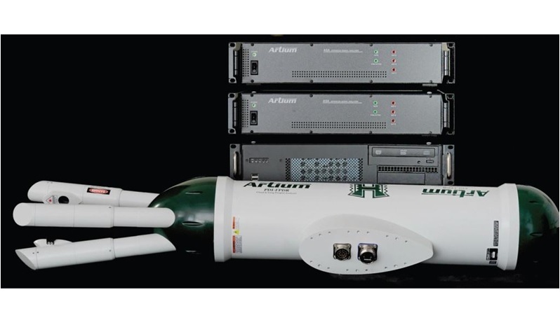
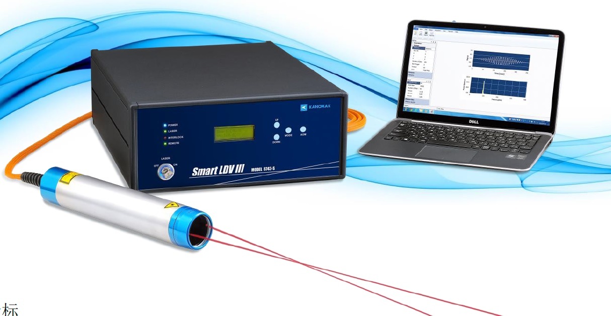

北京欧兰科技发展有限公司为您提供《云层中的水滴中水滴直径和速度分布检测方案(干涉仪)》,该方案主要用于航天中水滴直径和速度分布检测,参考标准《暂无》,《云层中的水滴中水滴直径和速度分布检测方案(干涉仪)》用到的仪器有激光相位多普勒干涉仪LDV,PDI,PDPA,PDA、Artium PDI-FP 双量程可机载飞行探头、紧凑型激光多普勒测速仪(LDV)、德国LaVision PIV/PLIF粒子成像测速场仪。
我要纠错
推荐专场
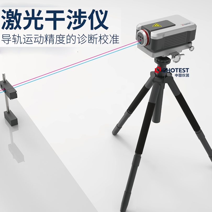
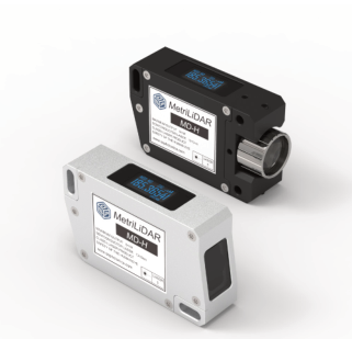
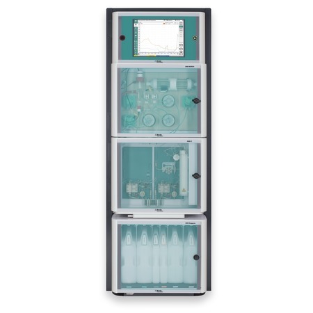
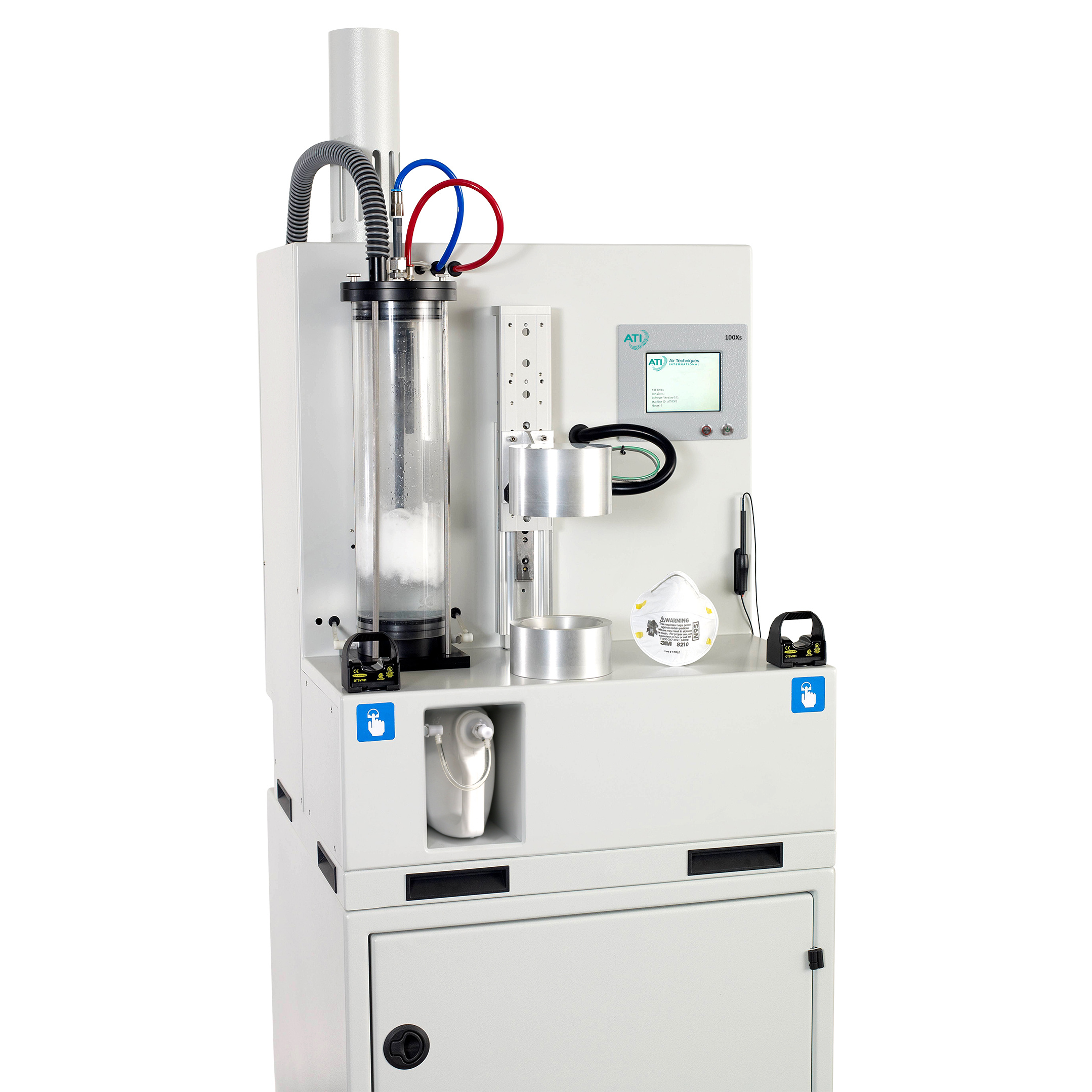


相关方案
 咨询
咨询