3D拉格朗日粒子追踪测速
检测样品
航空
检测项目
速度矢量场
关联设备
共2种
下载方案
方案详情文
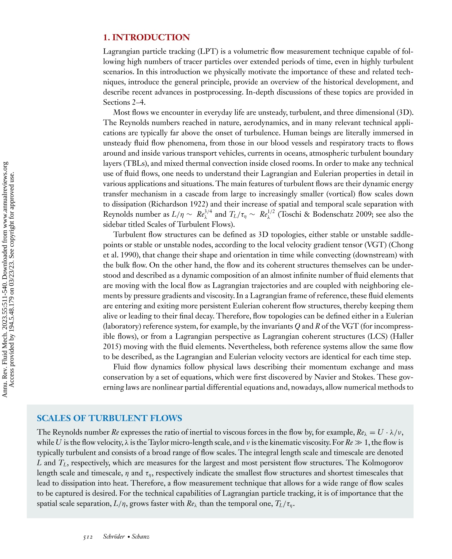
在过去几十年中,已经发展出了多种基于粒子图像的体积流场测量技术,这些技术已经在流体力学的各种实验应用中展示了它们量化评估非定常流动性质的潜力。在这篇综述中,我们专注于3D基于粒子的测量的物理特性和环境,以及可以用于提高重建精度、空间和时间分辨率以及完整性的知识。我们关注的自然候选者是3D拉格朗日粒子跟踪(LPT),它允许在所研究的体积中确定位置、速度和加速度以及大量单个粒子轨迹。过去十年中,密集的3D LPT技术“Shake-The-Box”的出现开辟了更多的可能性,通过提供用于使用Navier-Stokes约束的强大数据同化技术的输入数据来表征非定常流动。因此,可以获得高分辨率的拉格朗日和欧拉数据,包括嵌入时间分辨的3D速度和压力场中的长粒子轨迹。
智能文字提取功能测试中
拉格朗日粒子跟踪(LPT)是一种体积流量测量技术,能够在长时间内跟踪大量示踪粒子,即使在高度湍流的情况下也能做到。在本介绍中,我们从物理上说明这些技术及其相关性的重要性,介绍其一般原理,概述其历史发展,并描述了后处理方面的最新进展。这些主题的深入讨论在第2至4节中提供。我们在日常生活中遇到的大多数流动都是非定常、湍流和三维的。在自然界、空气动力学和许多相关的技术应用中达到的雷诺数通常远高于湍流发生的临界值。人类从字面上说是沉浸在非定常的流体流动现象中,从我们的血管和呼吸道中到各种交通工具内部和周围的流动、海洋中的洋流、大气湍流边界层(TBLs)以及封闭房间内的混合热对流。为了在各种应用和情况下充分利用流体流动,需要详细了解它们的拉格朗日和欧拉特性。湍流流动的主要特征是其动态能量转移机制,从大流动尺度向越来越小的(旋涡)流动尺度级联到耗散(Richardson 1922),并且随着雷诺数的增加而增加空间和时间尺度的分离,例如L/η ∼ Re3/4λ和TL/τη ∼ Re1/2λ(Toschi和Bodenschatz 2009;另请参见名为“湍流流动尺度”的侧栏)。根据局部速度梯度张量(VGT)(Chong等,1990),湍流流动结构可以定义为3D拓扑,即稳定或不稳定的鞍点或稳定或不稳定的节点,其在时间上改变形状和方向,同时随着整个流体流动(向下游)传导。另一方面,流动及其相干结构本身可以被理解和描述为几乎无限数量的流体元素的动态组成,这些元素沿着拉格朗日轨迹与局部流一起移动,并通过压力梯度和黏度与相邻元素耦合。在拉格朗日参考系中,这些流体元素正在进入和退出更持久的欧拉相干流结构,从而使它们保持活跃或导致它们的最终衰减。因此,流动拓扑可以在欧拉参考系(例如,通过VGT的Q和R不变量描述不可压缩流动),或者从拉格朗日视角作为与流体元素一起移动的拉格朗日相干结构(LCS)(Haller 2015)来定义。尽管如此,两个参考系都允许描述相同的流动,因为每个时间步长的拉格朗日和欧拉速度向量是相同的。Figure 2 (Figure appears on preceding page) Time-resolved multicamera recordings Annu. Rev. Fluid Mech. 2023.55:511-40 First published as a Review i n Advance on October 13,2022 The Annual Review of Fluid Mecbanics is online at fluid.annualreviews.org https://doi.org/10.1146/annurev-fluid-031822-041721 Copyright O 2023 by the author(s). This work is licensed under a Creative Commons Attribution 4.0International License, which permits unrestricted use, distribution, and reproduction in any medium,provided the original author and source are credited.See credit l ines of images or other third-party material in this article for license information. ANNUAL REVIEWS CONNECT www.annualreviews.org ·Down l oad figures ·Navigate c ited references · Keyword search · Explore related ar t icles · Share via email or social media Annual Review of Fluid Mechbanics 3D Lagrangian Particle Tracking in Fluid Mechan i cs Andreas Schroder1,2 and Daniel Schanz lInstitute of Aerodynamics and Flow Technology, Deutsches Zentrum f ur Luft- u nd Raumfahrt (DLR), Gottingen, Germany; email: andreas.schroeder@dlr.de 2Institute for Traffic Engineering , Brandenburgisch Technische Universitat (BTU) Cottbus-Senftenberg, Cottbus, Germany Keywords 3D particle tracking velocimetry, iterative particle reconstruction,Shake-The-Box, one- and multipoint s tatistics, velocity gradient t ensor,3D pressure fields, data assimilation Abstract In the past few decades various particle i mage-based volumetric flow mea-surement techniques have been developed that have demonstrated their potential in accessing unsteady flow properties quantitatively in various POt experimental applications i n fluid mechanics. In this review, we f ocus on physical properties and circumstances of 3D part i cle-based measurements and what knowledge can be used for advancing reconstruction accuracy and spatial and temporal resolution, as well as completeness. The natural candi-date for our focus i s 3D Lagrangian particle tracking (LPT ), which allows for position, velocity, and acceleration to be determined alongside a l arge number of individual particle tracks in the i nvestigated volume. The ad-vent of the dense 3D LPT technique Shake-The-Box in the past decade has opened further possibilities for characterizing unsteady flows by delivering input data for powerful data assimilation techniques that use Navier-Stokes constraints . As a result, high-resolut i on Lagrangian and Eulerian data can be obtained, including long particle t rajectories embedded i n time-resolved 3D velocity and pressure fields. 1. INTRODUCTION Lagrangian particle tracking (LPT) is a volumetric f low measurement technique capable of fol-lowing high numbers of tracer particles over extended periods of time, even in highly t urbulent scenarios. In this introduction we physically motivate the importance of these and related tech-niques, introduce the general principle, provide an overv i ew of the historical development, and describe recent advances in postprocessing. In-depth discussions of these t opics are provided in Sections 2-4. Most f lows we encounter in everyday l i fe are unsteady, turbulent , and three dimensional (3D).The Reynolds numbers reached in nature, aerodynamics, and i n many relevant t echnical appli-cations are typically f ar above the onset of turbulence. Human beings are literally i mmersed in unsteady fluid flow phenomena, from those in our blood vessels and respiratory t racts to flows around and inside various transport vehicles, currents in oceans, atmospheric turbulent boundary layers (TBLs), and mixed therma l convection i nside closed rooms. In order to make any technical use of fluid flows, one needs to understand their Lagrangian and Eulerian propert i es in detail in various applications and situations. The main f eatures of turbulent f l ows are their dynamic energy transfer mechanism in a cascade from l arge to i ncreasingly smaller (vortical) flow scales down to dissipation (Richardson 1922) and their increase of spatial and temporal scale separation with Reynolds number as L/n~ Re’4 and T/t~ Re (Toschi & Bodenschatz 2009; see also the sidebar titled Scales of Turbulent Flows). Turbulent flow structures can be defined as 3D topologies, either s table or unstable saddle-points or stable or unstable nodes, according to the local velocity gradient tensor (VGT) (Chong et al . 1990), that change their shape and orientation in t i me while convecting (downstream) with the bulk flow. On the other hand, the flow and its coherent structures t hemselves can be under-stood and described as a dynamic composition of an almost i nfinite number of fluid elements that are moving with the local flow as Lagrangian trajectories and are coupled with neighboring ele-ments by pressure gradients and viscosity. In a Lagrangian frame of reference, these fluid elements are entering and exiting more persistent Eulerian coherent f low s tructures, thereby keeping them alive or leading to t heir final decay. Therefore, flow topologies can be defined either i n a Eulerian (laboratory) reference system, for example, by the invariants Q and R of the VGT (for incompress-ible flows), or from a Lagrangian perspective as Lagrangian coherent structures (LCS) (Haller 2015) moving with the fluid elements. Nevertheless, both reference systems allow the same flow to be described, as the Lagrangian and Eulerian velocity vectors are i dentical for each time step. Fluid f low dynamics follow physical l aws describing their momentum exchange and mass conservation by a set of equations, which were first discovered by Navier and Stokes. These gov-erning laws are nonlinear partial differential equations and, nowadays, allow numerical methods to predict flows and their features by computer simulations, such as for aerodynamical design purposes. At high Reynolds numbers, the resolution requirements in space and time and the non-linearity of the flow physics involved pose many problems for numerical codes, regarding either the available computer resources or the validity and applicability of established turbulence mod-els or scaling laws (Mani & Dorgan 2023). A very high degree of computational effort i s already needed for predicting turbulent flows at moderate Reynolds numbers by direct numerical sim-ulations (DNS). Today, even with modern high-performance computing resources, converged DNS results (e.g., for the flow around a small passenger aircraft) cannot be provided at all and will most probably not be reachable within the next couple of decades. Therefore, (advanced)computational fluid dynamics code developments that use turbulence or subgrid-scale models to solve their c l osure problem [large eddy simulations, (unsteady) Reynolds averaged Navier-Stokes (NS) equations, etc.] require spatially (and temporally) well-resolved experimental validation data at high Reynolds numbers, preferably in f ull volumes around various model geometries. High-quality velocity vector f ields (instantaneous and mean with Reynolds stresses) enable the tuning of numerical parameters and the adaptation or further development of various t urbulence mod-els. Promising fields that will be closely l inked to velocity, acceleration, and pressure data from 3D LPT measurements in the near future include data-driven turbulence models (Duraisamy et al.2019) and the exploration of universal constants (Viggiano et al. 2021) or turbulent t ransport properties in inhomogeneous turbulence from Lagrangian s tatistics. 1.1. Particle Image-Based Velocimetry During the past decades a tremendous increase of flow field information has been gained from ex-perimental investigations applying image-based measurement techniques. Particle image-based methods visualize the flow using clouds of small tracer particles that are illuminated and observed by one or more cameras (complementary or alternative to existing probe techniques). For exper-iments in unsteady and turbulent f lows, nonintrusive volumetric and t i me-resolved measurement techniques, determining al l three components of the velocity (and acceleration) vectors at many points instantaneously, are highly desired. Consequently, i n recent years particle image velocime-try (PIV) techniques have been extended from 2D to 3D and from two-pulse snapshot modes to temporal resolution (Adrian & Westerweel 2011, Raffel et al. 2018, Beresh 2021). Various vol-umetric (and time-resolved) PIV and particle tracking velocimetry (PTV) techniques and their capabilities have already been presented in dedicated papers. For single (or stereo) camera views,scanning PIV has been proposed by, for example, Gray et al . (1991) and Brucker (1997); holo-graphic PIV techniques have been presented by Hinsch (2002), Katz & Sheng (2010), and others;coded aperture PIV was first introduced by Willert & Gharib (1992); defocusing PIV was de-scribed by Pereira et al . (2000); structured-light PIV was described by, e.g., Aguirre-Pablo et al.(2019); and light field or plenoptic PIV was described by Fahringer et al. (2015) and others. Appli-cations of single-camera 3D PTV for microfluidics include astigmatism (Cierpka et al. 2010) and holographic PTV (Choi et al. 2012). Single-view 3D PIV and PTV techniques can operate with less optical access, but due to the l imited aperture, the reconstructed particle position uncertainty in depth direction (the direction parallel to the main viewing direction of the camera) is much larger (typically by a factor greater than 3) compared to the in-plane uncertainties. Multicamera methods rely on several camera projections, allowing similar position and velocity uncertainties in al l three directions in space when appropriate projection angles are applied (ideally an angle of 90° is used between the two outermost cameras-the “aperture”of the camera system). Tomographic PIV (Tomo-PIV), which was introduced by Elsinga et al. (2006) and further developed by Wieneke (2008), Atkinson & Soria (2009), and Novara et al. (2010), significantly Particle i mage velocimetry (PIV): flow measurement method for obtaining 2D fields of veloc i ty vectors by cross-correlat i ng subsequent images of tracer particles Particle image density, Nr: measure to describe the density of particle image peaks on a camera i mage;expressed in part i cles per pixel (ppp) Ghost particle: falsely reconstructed 3D particle (position) that does not exist in the originally imaged part i cle cloud Peak: image of a single particle on a camera,typically a (distorted)Gaussian with a diameter of 2-3 pixels Line-of-sight (LOS):the viewing path through the measurement region of a given camera image coordinate, as given by the calibration enhanced the spatial resolution of volumetric velocimetry. Therefore, Tomo-PIV rapidly evolved to become the most commonly used and robust 3D flow measurement technique in the decade following its first publication. It enables flow field estimates to be delivered on regular 3D velocity vector grids via iterative local cross-correlation schemes with relatively high spatial resolution based on, typically, four to six camera projections and at particle image densities around Nr=0.05particles per pixel (ppp). Furthermore, by using many camera projections one can i ncrease the number of truly reconstructed particles per t ime step while reducing t he so-called ghost particle fraction (Elsinga et al . 2006), which holds true as well for particle-based reconstruction schemes for 3D LPT. For all 3D reconstruction techniques, Nr determines the possible spatial resolution i nside the investigated flow for a given depth of t he measurement volume; however, the reconstruction dif f iculty increases with N. The maximum value of Nr at which a method can reliably reconstruct true part i cles while not creating too many ghost particles typically determines i ts performance.Novel machine l earning (ML) approaches are promising methods for increasing t he range of N-values for Tomo-PIV techniques (Gao et al . 2021). A further i ncrease of spatial resolution or particles per volume (ppv) has been achieved by a scanning Tomo-PIV setup in a turbulent l ow-speed flow (Lawson & Dawson 2014). However, for all cross-correlation-based PIV techniques,a spatial low-pass filter modulation of the velocity gradients inside the measured f low has to be accepted because only a group of particle images (typically four to ten) located i nside a 2D or 3D correlation window [e.g., 322px (pixels) or 323 voxels] enables a robust estimation of the position of t he local displacement vector peak. Furthermore, acceleration vector fields are not di r ectly accessible by this method. Consequently, a measurement technique that enables i ndividual t racer particles to be followed volumetrically and at high densities i n t ime i s more suited to bridge the scattered measurement data, i ncluding position, velocity, and acceleration, along reconstructed particle t rajectories to the governing NS equations. px: normalized l ength of a camera pixel,scaled by the average magnification; it is thereby a universal measure for comparing 3D i maging systems 1.2. Particle Trackin g M ethods In contrast to PIV methods, particle tracking methods have been developed with 3D PTV schemes that enable relatively sparse particle track reconstructions (e.g., Nishino et al. 1989, Maas et al.1993, Malik et a l . 1993, Guezennec et al. 1994, Virant & Dracos 1997, Ouellette et al. 2006,Machicoane et al . 2019, Dabiri & Pecora 2020) at particle image densities between ~0.005 and 0.02 ppp. Increased particle track densities in the measurement volume can be achieved with scan-ning 3D PTV techniques (Hoyer et al. 2005, Kozul et al. 2019), reaching higher ppv values for relatively low flow velocities. Nowadays, state-of-the-art 3D LPT techniques can reach high par-ticle image densities of ~0.05-0.2 ppp using the Shake-The-Box (STB) method (Schanz et al.2016,Jahn et al. 2021, Leclaire et al . 2021, Sciacchitano et al.2021b). Figure 1 depicts the general working principle of 3D particle tracking experiments: First, par-ticle images of (illuminated) passive tracers inside the flow are taken simultaneously f rom several camera projections (typically three to six) for each time step. Then, particle image peaks are de-tected on each camera and the l ines-of-sight (LOS) of each peak are virtually elongated into t he measurement volume according to the 3D camera calibration. When LOS of detected particle image peaks on several cameras i ntersect below an allowed t r iangulation error (~1 px), a t rue 3D particle position can be assumed. Using all detected peaks on the different cameras, one can recon-struct clouds of 3D particle positions for each time step. A tracking approach is then applied in a second step that aims at always f inding the identical imaged particle along the corresponding time-line of 3D particle reconstructions in order to build up long 3D particle trajectories. The actual implementations of the different LPT steps can be performed with varying levels of sophistication and are discussed in Sections 2 and 4. Reconstruction: 3D positions from 2D peaks using calibrated l ines-of-sig ht Figure 1 The basic steps of a Lagrangian particle t racking experiment. 2D particle i mages (peaks) are identified on all camera images for a certain t ime step (green dots) and then used to determine 3D positions (blue dots) using (iterative) triangulation procedures (red lines). The particle clouds from several t ime steps can be connected to tracks under certain constraints. Velocity and acceleration of the trajectories yield several properties via postprocessing (e.g., flow structures) by applying regularized interpolation (data assimilation) to all particles tracked at a certain time step. Figure 2 shows a specific application of LPT i n a large and densely seeded Rayleigh-Benard convection cell. The key aspects of the setup are a pulsed volumetric illumination and a multicam-era setup consisting of at least three cameras and capable of temporally resolving the flow. Here,the STB algorithm (see Section 3.1) was used to i nstantaneously track up to 560,000 tracers over long periods of time from the images obtained from six cameras (Bosbach et al. 2021, Godbersen et al. 2021). Here we would like to sugges t using the name “3D LPT”for volumetric measurements ofindi-vidual particle trajectories (following, e.g., Ouellette et al. 2006) because t he achievable measures along individual particle paths are manifold, including position, velocity, acceleration (material derivative), and (sometimes even) j erk, as well as t heir Lagrangian properties. All of these are important for the f luid mechanical characterization of the investigated flow and are valuable i n-puts for high-resolution postprocessing approaches using bin-averaging for one- and multipoint statistics, data assimilation (DA), ML, and integration [e.g., pressure from LPT (Rival & van Oudheusden 2017, van Gent et al. 2017)]. The velocity , as might be suggested by t he t erm“PTV,”is not the only i mportant outcome. Tomo-PIV and 3D LPT/PTV techniques, as well as various similar volumetric velocimetry techniques for f luid flows, have been extensively presented and discussed i n recent reviews (e.g.,Scarano 2013, Westerweel et al . 2013, Discetti & Coletti 2018, Machicoane et al. 2019) and text-books (Schroder & Willert 2008, Adrian & Westerweel 2011, Raffel et al. 2018, Dabiri & Pecora 2020). Furthermore, with the recent development of high-speed l asers and cameras, the range of flow velocities i n which time-resolved velocity field information can be gained via PIV and LPT has been widened significantly in spatial and temporal resolution (Beresh 2021). In all various volumetric flow measurement techniques, the achievable dynamic spatial range (DSR) (see Adrian 1997) for sampling any (turbulent) f low f ield is mainly rest r icted by the res-olution of the used camera sensor and the reachable volumetric particle density, which l imit the Data assimilation (DA): the process of combining measurement data (e.g., particle position, Tracking of ≈560,000 tracers Q-criterion from FlowFit in the ful l RBC volume int e rpolation of tracks (a) Exemplary setup of a Lagrangian particle tracking (LPT) experiment, consisting of a Rayleigh-Benard convection (RBC) cell 1.1 m in height with tracer particles (here, helium-filled soap bubbles) illuminated by a pulsed light source (here, f rom above by arrays of high-power LEDs (light-emitting diodes) shining through a transparent water-cooled top plate). The i lluminated tracers are r ecorded in a time-resolved f ashion by a system of cameras, all i maging the same (illuminated) volume. (b) Actual i mage f rom one camera of t he experiment , showing bubbles i nside the cell and the illuminated heated floor. The i nsets show examples at several particles per pixel (ppp) concentrations. (c) LPT was performed on the high-density i mages using the Shake-The-Box method. (d) Flow structures can be visualized by applying FlowFit data assimilation to the tracked part i cle field in panel c. Panels adapted from Godbersen et al. (2020)(CC BY-NC 4.0; https://doi.org/10.1103/APS.DFD.2020.GFM.V0074). instantaneous sampling of the l argest and smallest achievable f low structures, respectively. The latter is directly related to Ni and the depth of the investigated volume. Therefore, if flow dy-namics and repetition rates of cameras and illumination allow, 3D scanning methods can achieve relatively high volumetric particle densities (and DSR values) and do not suffer (like many other techniques) from both the reduction of scattered particle l ight due to smal l camera l ens apertures and the expansion of the available (laser) light for full volumetric i llumination. On the other hand, the dynamic velocity range (DVR) (Adrian 1997) and dynamic accelera-tion range (DAR) (Schanz et al. 2016) are strongly linked to the reconstructed particle position accuracy and the temporal sampling along the (exploitable) particle trajectories. To enhance DSR and DVR of particle-based measurements , the need for a “completely new approach”has already been proclaimed (Westerweel et al . 2013,p. 409). In general, multi-illumination or t ime-resolved imaging strategies of tracer particles inside f lows enable higher accuracies t han can be achieved with two-pulse strategies when determining temporal derivatives of the particle trajectory. All three characteristic values, DSR, DVR, and DAR, can be maximized in a 3D LPT experiment by exploiting the knowledge of the physical (fluid mechanical and optical) properties of the i ndi-vidual tracer particles and their imaging. Applying this physical knowledge for an enhanced 3D particle reconstruction and tracking scheme was the path followed by the STB development i n the past decade. High position accuracies of reconstructed particles require well-sampled particle images (~2 px i n diameter, no pixel-locking) at high signal-to-noise ratio (SNR), as the discret i zed gray values of particle i mages contain the particles’ posit i on i nformation. Then, the applied 3D reconstruction scheme should aim at a strong reduction of ghost part i cles i n order to keep the distributed i mage intensity at the true particles’ positions for enhancing their position accuracy.Finally, having obtained such high positional accuracies, accurate temporal derivatives along f itted tracks, like velocity and acceleration, are only available at sufficiently high sampling frequencies.With respect to extreme but rare acceleration events inside turbulent flows, it has been proposed that one samples at l east 40 times faster than the Kolmogorov t imescales, t ,, in order to avoid respective t racking and truncation errors (Lawson et al. 2018). However, hardware restrictions do not always allow for such high illumination and i maging frequencies. In Section 3.2 below the temporal sampling problem for high-acceleration (and -jerk) events i s addressed again in the context of an advanced prediction and correction STB scheme. 1.3. Advanced 3D Particle Tracki ng a nd Data Assimilation Techniques The STB technique is an advanced 3D LPT method t hat combines the triangulation-based ad-vanced iterative part i cle reconstruction (IPR) technique (Wieneke 2012,J ahn et al. 2021) with t he exploitation of the temporal and spatial coherence of Lagrangian part i cle tracks i n the i nvestigated flow. STB enables the processing of particle i mage densities up to Nr=0.2 ppp under good ex-perimental conditions with an almost complete suppression of ghost particles. Subsequently, the dense scattered particle tracks are temporal l y filtered (Gesemann et al. 2016, Gesemann 2021) for estimating position, velocity, and acceleration (material derivative), which can be used in a second step as input for DA approaches using NS constraints, delivering the f ul l time-resolved 3D veloc-ity gradient tensor and pressure fields (e.g., Gesemann et al . 2016, Schneiders & Scarano 2016,Jeon 2021). Using only solenoidal constraints applied to dense LPT data, in case D of the Fourth International PIV Challenge in 2014, the first DA schemes hav e already shown better spatial and temporal resolution of the reconstructed volumetric flow f ield than advanced Tomo-PIV tech-niques (see Kahler et al. 2016). A f urther benchmark test of the 3D pressure f ield reconstruct i on capabilities of various pressure from PIV and LPT approaches also showed strong benefits in us-ing dense LPT data, delivering velocity and acceleration vector f ields as i nput f or DA schemes that apply fully nonlinear NS constraints (see van Gent et al. 2017). Current developments aim at maximizing the achievable flow information from s ingle flow experiments at high particle im-age densities by applying (combined) 3D LPT, DA, and ML (Brunton et al. 2020) approaches.However, in many high-speed flow experiments, ful l temporal resolution for particle i mage-based volumetric velocimetry is still not possible. Here, multipulse and multi-illumination techniques for Tomo-PIV (Lynch & Scarano 2014, Schroder et al. 2013) and LPT (Novara et al. 2016b,2019)have been developed that can capture volumetric velocity f ields at high spatial resolution, as well as DVR (see Figure 5) (e.g., van Gent et al. 2017). The scattered nature of the individually tracked partic l es provides a great advantage over other related measurement techniques such as PIV. Instead of a fixed regular grid of convolution win-dows whose size imposes a low-pass filtering effect on resolvable flow structures and gradients,the particle track positions are distributed homogeneously and provide l ocal point measurements of f luid elements when using particles with diameters below the smallest scales of the investi-gated flows, such as the Kolmogorov length scale dp When the process of particle tracking i s f inished, the tracks consist of raw particle positions for all t ime steps. A temporal f ilter i s used to increase the positional accuracy and to extract the Lagrangian velocity and acceleration (see Figures 2c and 6, as well as the left and middle of Supplemental Video 1). To this end, various methods are applicable. A polynomial f it of second or third order can be applied,with the possibility oftuning the filter strength to the experiment via the length of the used kernel. This kernel can even be dynamically adapted to the current state of t he particle (Janke & Michaelis 2021). Another approach is the use of a (cubic) B-spline curve whose filter strength can be calibrated to the noise conditions by deducting a crossover f requency f rom the position amplitude spectrum, which also yields the average position accuracy (Gesemann et al.2016, Gesemann 2021). The method can be tuned to be equivalent to an optimal Wiener filter.As a rule of thumb, the positional errors can be nearly halved by applying a well-calibrated f ilter. 4. POSTPROCESSING OF LAGRANGIAN DATA LPT methods s imultaneously yield long Lagrangian t rajectories for a multitude of particles and a discrete f ield of velocity and acceleration information at the particle locations for each time step, and even in between them, given the continuous f iltering. This allows one to go beyond the diffraction l imitation of particle imaging for t wo-point statistics (Godbersen & Schroder 2020, Hammond & Meng 2021). A broad field of research to benefit from such enhanced 3D LPT methods is particle-laden turbulence, especially when collisions need to be considered Exemplary measurement using Mult i -Pulse STB: A TBL f low with a micrometer-sized droplet seeding is illuminated by two double-pulse lasers (80×120×10 mm’) and observed by eight double-frame cameras, illuminating each frame twice. From each image pair, approximately 95,000 part i cles are t racked. This data can be used, for example, by dat a assimilation for flow structure identification or by bin-averaging methods to determine high-resolut i on profiles of velocity and Reynolds stresses. Figure adapted f rom Novara et al . (2019), with permission from Springer; copyright 2019 Springer-Verlag. Abbrev i ations: DNS, direct numerical simulation; STB, Shake-The-Box; TBL, turbulent boundary layer. (Brandt & Coletti 2022). Inertial particles (Ebrahimian et al. 2019) and slip over superhydrophobic surfaces (Abu Rowin & Ghaemi 2019) i n turbulent boundary l ayers have been investigated using STB. Besides t he creation of highly resolved Lagrangian and Eulerian statistics, the t racking data may be used in various ways, as described below. 4.1. Bin Averaging Advanced binning procedures can produce a 3D array of one-, two-, a nd multipoint statistics of the flow (mean values, Reynolds stresses, two-point correlations, structure functions, etc.)at very high spatial resolution, down to subpixel accuracies. According to Reynolds (triple) Figure 6 Lagrangian part i cle tracking measurement in homogeneous turbulence at Rex=270 in a von Karman water f low between two counter-rotating propellers (Schroder et al . 2022).(a) Approximately 65,000 particles v i sualized at five consecutiv e t ime steps as spheres, colored by x-velocity.(b) The s ame flow situation, here with 30 t ime steps, connected by velocity vectors and colored by x-acceleration (ax). (c) Flow structures identified via FlowFit data assimilation of the particle cloud at the central time step, given by an isosurface of the Q-criterion (Q=2,500/s²). decomposition,u= u(+it)+ u’, the statistical f low quantities are the mean u (periodic i t) and f luc-tuation u’ components of all three velocity vector components. The respective Reynolds stress tensor u'u, and higher-order statistics are further measures for characterizing unsteady and turbu-lent flows. Profiles of these quantities can be determined by dividing the measurement region into 3D bin averaging of the flow around a cube mounted on a surface and submerged in a laminar boundary layer wit h a f low speed of U = 0.2 m/s and a bin size of 0.25×0.25×0.25 mm’ (see Schroder et al. 2020). small subregions (bins) and averaging the properties of all particles located within each of these bins over all measurements available. Depending on the flow and the volume, the profiles can be 1D, 2D, or 3D. Figure 7 shows a 3D-averaged profile of the flow around a surface-mounted cube,while Figure 5 displays a 1D profile of Reynolds stresses of a TBL with a resolution of 14.5 um (1/3 of a viscous unit). The usable size of t he bins scales i nversely wi t h the number of measure-ments: The more data that are available, the f iner the resolution can be (in contrast to PIV, which is always limited to the correlation window size). Important for the reliability of the statistics is a local convergence study and a precise uncertainty quantification. Recent l y, a versat i le f unctional bin-ning procedure has been i ntroduced that optimizes the convergence speed of 3D LPT one-point and multipoint statistics by using the continuous track and uncertainty information (instead of sampling t he particle only at each measured time step) (Godbersen & Schroder 2020, Godbersen & Schroder 2021). Further measures to increase the spatial resolution have been integrated i nto the functional approach, such as arbitrarily shaped bins (Raiola et al. 2020) and weights, allowing for adaptation to mean flow gradients (Aguiera et al. 2016). 4.2. Data Assimilation for Spatial Interpolation Representing flow data on a regular grid or in a continuous functional way within a Eulerian frame of reference is desirable for many established processing methods (e.g., for f low structure identification and pressure determination). The availability of Lagrangian velocity and acceler-ation allows for interpolations that go beyond a simple averaging approach. In t he l ast couple of years, techniques for DA schemes have been established for s ingle- and multi-timestep LPT results using solenoidal constraints or a full i ncompressible NS regularization. For the latter,velocity and acceleration (material derivative or left side of t he NS momentum equation) are used Di(2-ethylhexyl)sebacate (DEHS):a l i quid used for the generation of aerosol particles, often used for laser-based fow measurements in air as i nput values. Such methods include FlowFit (Gesemann et al . 2016) and vortex-in-cell (VIC)approaches [VIC+ (Schneiders & Scarano 2016), VIC# (Jeon et al. 2018, Jeon 2021), and VIC-TSA (Scarano et al. 2022)]. These DA schemes provide a continuous functional representation of the assimilated velocity vector field without additional spatial f iltering, on the basis of (truncated)3D radial basis functions or third-order B-splines. Analytical derivat i ves can be computed for the full t ime-resolved velocity gradient tensor Aij(t) for an arbitrary grid, and 3D pressure f ields are i mplicitly integrated by solving the related Poisson equation and imposing constraints from t he i n-compressible NS equations using nonlinear optimization solvers [e.g., L-BFGS (limited-memory Broyden-Fletcher-Goldfarb-Shanno) (Nocedal 1980; see also van Gent et al. 2017, Huhn et al.2018)]. In their review on the development of load estimation techniques, Rival & van Oudheusden (2017) explicitly proposed that LPT+DA will become the new standard for i nstantaneous 3D pressure reconstruction and stated i ts i mportance for future measurements of unsteady flows.Examples of DA applied to LPT data can be found in Figures 2d, 5, and 6c, as well as in Supplemental Video 1 (right panel). Supplemental Material 1> 5. LARGE-SCALE VOLUMETRIC MEASUREMENTS For a long time during the development of PTV and Tomo-PIV, volumetric i nvestigations r e-mained limited to relatively small volumes. High-speed lasers were used to i l luminate DEHS [di(2-ethylhexyl) sebacate] droplets (~1 um in diameter) in air or suitable tracers in water (e.g.,polyamide particles up to 100 pm in diameter, depending on the scales to be resolved). Especially in air, the smal l tracers restricted the volumes that could be i l luminated to a few cubic centime-ters . Two developments changed this: the steady progress i n t he development of LEDs, allowing researchers to build scalable pulsed i llumination arrays (Stasicki et al. 2017), and the i ntroduct i on of submillimeter HFSB t racer particles in air (Bosbach et al. 2009). The l ight reflected on the ~300-um-diameter bubbles is orders of magnitude more intense t han the l ight scattered on s mall oi l droplets. At the same time, density matching ensures a high f low-tracing f idelity (Scarano et al.2015). With laser illumination, the applicable volume size for high-speed investigations grows to several liters (Scarano et al.2015); for LED illumination, the volume is mostly limited by the number of available LEDs. First attempts by Kuhn et al. (2011) used Tomo-PIV in a convection cell with 55 liters of measured volume. The i maging properties of the (noncoherent) l ight re-flected on t he bubbles proved to be very favorable for particle t racking methods. Time-resolved investigations of an impinging jet (Huhn et al. 2018) and a turbulent boundary l ayer (Schanz et al.2019) have also been performed. The latter reached a volume size of 450 liters. When i nvestigat-ing slow flows (e.g., driven by temperature gradients), one can use illumination times of several milliseconds , further increasing the achievable volume size. A thermal plume has been captured in a volume of 550 l iters (Huhn et al.2017), and the Rayleigh-Benard flow depicted i n Figure 2was measured in 1,045 liters, the f ull volume of the cell. Recently, a f low measurement around a breathing and heated human model was performed i n a volume of 12 m’(Schroder et al. 2022).The use of high-resolution cameras allowed up to 3 million bubbles to be followed i nstantaneously and small instantaneous turbulent structures of the thermal plume to be resolved, despite the l arge volume size. Scalable LED illumination has also been applied in water, yielding images free of ar-tifacts caused by coherent l ight (Kim et al. 2021). The image quality can be further improved by using f luorescent particles and appropriate filters (Kim et al . 2022, Weiss et al. 2022). A different approach to increasing the volume size was developed by Schneiders et al . (2018)in the form of the coaxial volumetric velocimeter. The measurement device consists of a f ixed and precalibrated system of four cameras, i nstalled i n a common housing. Between t he cameras a volumetric laser illumination is i nstalled (Figure 8a). The l ight reflected by HFSB seeding is Figure 8 A coaxial volumetric velocimeter for time-averaged l arge-volumetric measurements. (a) Lavision's MiniShaker S consists of a f ixed and precalibrated system of four cameras, installed i n a common housing.(b) Measurement of a single subvolume i n front of a cyclist.(c) Scanning of the ful l volume using a robotic arm. (d) Time-averaged velocity f ield around full cyclist model, showing contours of streamwise velocity u in the center plane, together with an isosurface of u=7 m/s. (e) Surface pressure coefficient Cp distribution in the foot/ankle region, along with isocontours of the Q-criterion,colored by streamwise vorticity w.. Panels a,c, and d adapted from Jux et al. (2018) (CC BY 4.0). Panels b and d adapted f rom Jux (2022) with permission; copyright 2021 t he author. Abbreviation: HFSB,helium-filled soap bubbles. recorded by the four cameras; particle trajectories are reconstructed using STB. The device can simply be pointed at a region of interest and operated for a certain time, yielding LPT results i n a volume of up to 30 liters (Figure 8b). Larger volumes are scanned by moving the velocimeter on a robotic arm, systematically scanning the object ofinterest (Figure 8c). One i nteresting application of the method i s the measurement of the f low around a full-scale cyclist (Jux et al . 2018), which yielded the flow i n a volume of 2 m’at a freestream velocity of 14 m/s by stitching together 450subvolumes (Figure 8d,e). Other examples include an investigation of the flow behind a micro air vehicle (Martinez Gallar et al. 2020) and the determination of all components in Collar’s triangle of forces acting on a flexible wing (Mertens et al. 2021). The downsides of t he method are the low position accuracy in the depth direction (due to the limited opening angle of the camera views)and the restriction to averaged data due to the scanning approach. SUMMARY POINTS 1. Lagrangian particle t racking (LPT) can accurately track a large number of particles (10+-10), yielding a high dynamic spatial range (DSR). Applying t emporal f iltering at calibrated levels yields high dynamic velocity and acceleration ranges (DVRs and DARs). 2. Recent developments in LPT software allow the usable particle i mage density con-centration to be increased by up to ~0.2 particles per pixel (ppp) using advanced Shake-The-Box (STB) processing-many times more than the densities reached by classical particle tracking velocimetry (PTV) methods. Furthermore, these advances have increased DVR significantly compared to two-pulse tomographic particle i mage velocimetry (Tomo-PIV) measurements. 3. The dynamics of a flow plays an important role in its evaluation. Regions of quiescent flow can be as problematic for the tracking scheme as rare high-accelerat i on events or low temporal sampling. The variable space step and variable time step methods i mprove the tracking performance of the STB scheme in such conditions. 4. High particle densities allow one to create converged single- and multipoint s tatistics at subpixel resolution (~0.1 px), greatly increasing the DSR for statistical approaches.Statistics for proximities below the diffract i on limits of imaging can be reliably determined using functional binning approaches. 5. Time-resolved 3D velocity, acceleration, and pressure fields represented by continuous 3D functions can be determined using novel constrained data assimilation (DA) methods (3D and 4D variational , as well as adjoint). The availability of velocity and accelera-tion (material derivative) data allows for Navier-Stokes constraints to be used, thereby achieving maximized spatial resolution from the dense scattered tracer particles. 6. The quality of LPT measurements is greatly dependent on the care t aken to optimize experimental parameters (e.g., image signal-to-noise ratio, particle scattering properties,available temporal resolution). Likewise, researchers should aim to guarantee a precise calibration at all t i mes using (instantaneous) volume self-calibration. Further correction methods can account for nonlinear effects (e.g., viewing t hrough curved windows). 7. The use of noncoherent l i ght sources (e.g., LED arrays) illuminating sufficiently l arge tracer particles (e.g., helium-filled soap bubbles in ai r , polyamide in water) produces particle imaging highly suitable for LPT evaluation in large volumes due to the much-improved superposition and consistency of particle images. Using f l uorescent particles additionally minimizes background reflections. FUTURE ISSUES 1. An enhanced predictor scheme could incorporate corrections using preknowledge of the flow topologies, gained either by computational fluid dynamics (CFD) or previous ex-perimental results. Further i mprovements are expected using DA of previous t ime steps,advected to the current time, creating a physics-based space-time link. 2. The effect of partic l e images overlapping in one or multiple cameras on position accuracy and local bias errors should be quantified. Generally, tools for uncertainty quant i fication of LPT and DA need to be further developed and assessed. 3. An openly accessible benchmark data set (HOMER LPT and DA Evaluation Portal;https://w3.onera.fr/flow-benchmarks) i s available and will be extended continuously,allowing researchers for the first time to quantitatively compare different methods on a common synthetic data base using underlying CFD s imulations. 4. A further significant increase of processable particle i mage densities will be difficult to achieve. However, higher particle concentrations (particles per volume) could be reached by using a scanning approach in low-speed flows, avoiding phase shifts by regarding t he trajectories as functionals. 5. Current DA approaches mainly apply regularization based on the momentum equation.Further constraints could be gained by using more conservation l aws and equations (e.g.,the energy equation) and by thoroughly utilizing the temporal resolution. 6. The prediction and correction scheme introduced by the STB method could also be implemented for other 3D flow measurement techniques like holographic, astigmatic,light field, and tomographic particle tracking. DISCLOSURE STATEMENT The authors are not aware of any biases that might be perceived as affecting the objectivity of this review. ACKNOWLEDGMENTS This work was partly supported by the Deutsche Forschungsgemeinschaft (DFG) through grant SCHR 1165/5-1/2 as part of the Priority Program on Turbulent Superstructures (DFG SPP1881,first and second period) and the HOMER (Holistic Optical Metrology for Aero-Elastic Research)project from the European Union’s Horizon 2020 research and i nnovation program under grant agreement 769237. The authors thank Matteo Novara and Tobias Jahn for valuable discussions and longstanding support. The help of Philipp Godbersen and Hicham Saaid i n the creation of the figures is greatly appreciated. LITERATURE CITED Abu Rowin W, Ghaemi S. 2019. Streamwise and spanwise slip over a superhydrophobic surface.7. Fluid Mecb.870:1127-57 Adrian RJ. 1997. Dynamic ranges of velocity and spatial resolution of particle i mage velocimetry. Meas. Sci.Tecbnol. 8(12):1393 Adrian RJ, Westerweel J. 2011. Particle Image Velocimetry. Cambridge, UK: Cambridge Univ. Press Aguera N, Cafiero G, A starita T , Discetti S. 2016. Ensemble 3D-PTV for high resolution t urbulent s tatistics.Meas. Sci. Tecbnol. 27:124011 Aguí JC, J imenez J. 1987. On the performance of particle tracking. J. Fluid Mecb. 185:447-68 Aguirre-Pablo AA, Aljedaani AB, XiongJ, Idoughi R, Heidrich W, Thoroddsen ST . 2019. Single-camera 3D PTV using partic l e i ntensities and structured l ight. Exp. Fluids 60(2):25 Atkinson C, Soria J. 2009. An efficient simultaneous reconstruction technique for tomographic part i cle image velocimetry. Exp. Fluids 47:563-78 Bhattacharya S, Vlachos PP. 2020. Volumetr i c particle t racking velocimetry (PTV) uncertainty quantification.Exp. Fluids 61(9):197 Beresh SJ. 2021. Time-resolved particle image velocimetry. Meas. Sci. Tecbnol. 32:102003 Bosbach J, Kuhn M, Wagner C. 2009. Large scale particle image velocimetry with helium filled soap bubbles.Exp. Fluids 46:539-47 Bosbach J, Schanz D, Godbersen P, Schroder A. 2021. Spatially and temporally resolved measurements ofturbu-lent Rayleigb-Benard convection by Lagrangian par t icle tracking of long-lived belium-filled soap bubbles. Paper presented at 14th International Symposium on Particle Image Velocimetry, Chicago, Aug. 1-4 Brandt L, Coletti F. 2022. Particle-laden turbulence: progress and perspectives. Annu. Rev. Fluid Mecb. 54:159-89 Bross M, Fuchs T, Kahler CJ . 2019. Interaction of coherent flow structures in adverse pressure gradient turbulent boundary layers. j. Fluid Mecb. 873:287-321 Brucker C. 1997.3D scanning PIV applied to an air f low in a motored engine using digital high-speed v i deo.Meas. Sci. Technol. 8:1480 Brunton SL, Noack BR, Koumoutsakos P. 2020. Machine learning for fluid mechanics. Annu. Rev. Fluid Mecb.52:477-508 Chiu WC, Rib LN. 1956. The rate of dissipation of energy and t he energy spectrum in a low-speed turbulent jet. Eos 37(1):13-26 Choi YS, Seo KW, Sohn MH, Lee SJ. 2012. Advances i n digital holographic micro-PTV for analyzing microscale flows. Opt. Lasers Eng.50(1):39-45 Chong MS, Perry AE, Cantwell BJ. 1990. A general classification of three-dimensional flow f ields. Pbys. Fluids A2(5):765-77 Cierpka C, Litke B, Kahler CJ. 2013. Higher order multi-frame part i cle t racking velocimetry. Exp. Fluids 54(5):1533 Cierpka C, Rossi M, Segura R, Kahler CJ. 2010. On the calibrat i on ofastigmat i sm particle tracking velocimetry for microflows. Meas. Sci. Tecbnol.22(1):015401 Cornic P, Leclaire B, Champagnat F, Le Besnerais G, Cheminet A, et al . 2020. Double-frame tomographic PTV at high seeding densities. Exp. Fluids 61(2):23 Dabiri D, Pecora C. 2020. Particle Tracking Velocimetry. Bristol, UK: IOP Discetti S, Coletti F. 2018. Volumetric velocimetry for f luid flows. Meas. Sci. Tecbnol. 29:042001 Doh DH, Cho GR, Kim YH. 2012. Development of a tomographic PTV.J. Mecb. Sci. Tecbnol.26(12):3811-19 Duraisamy K, Iaccarino G, Xiao H. 2019. Turbulence modeling i n the age of data. Annu. Rev. Fluid Mecb.51:357-77 Ebrahimian M, Sanders RS, Ghaemi S. 2019. Dynamics and wall collision of inertial particles in a solid-liquid turbulent channel flow. j. Fluid Mecb. 881:872-905 Elsinga GE, Scarano F, Wieneke B, van Oudheusden BW. 2006. Tomographic part i cle i mage velocimetry.Exp. Fluids 41:933-47 Fahringer TW, Lynch KP, Thurow BS. 2015. Volumetric particle i mage velocimetry with a s ingle plenoptic camera . Meas. Sci. Tecbnol. 26:115201 Fletcher R, Powell M. 1963. A rapidly convergent descent method for minimization. Comput.7.6(2):163-68 Fuchs T, Hain R, Kahler CJ. 2016. Double-frame 3D-PTV using a tomographic predictor. Exp. Fluids 57:174 Gao Q, Pan S, Wang H, Wei R, Wang J. 2021. Particle reconstruction of volumetric particle i mage velocimetry with the strategy of machine learning. Adv. Aerodyn. 3:28 Geisler R,Novara M, Schroder A. 2016. Volumetric multi-pulse particle tracking measurement f or s eparated laminar transitional flow investigations. Paper presented at 18th Internat i onal Symposium on Applicat i on of Laser and Imaging Techniques to Fluid Mechanics, Lisbon, Port ., J uly 4-7 Gesemann S. 2021. TrackFit: uncer t ainty quantification, optimal filtering and i nterpolation of tracks for time-resolved Lagrangian par t icle tracking. Paper presented at 14th International Symposium on Particle Image Velocimetry, Chicago,Aug. 1-4 Gesemann S, Huhn F, Schanz D, Schroder A. 2016. From noisy particle tracks to velocity, acceleration and pressure fields using B-splines and penalties. Paper presented at 18th International Symposium on Application of Laser and Imaging Techniques to Fluid Mechanics, Lisbon, Port., J uly 4-7 Godbersen P, Bosbach J, Schanz D, Schroder A. 2020. The beauty of t urbulent convection: a particle tracking endeavor. Film presented at Gallery of Fluid Mot i on, 73rd Annual Meeting of the APS Division of Fluid Dynamics (Virtual), Nov. 22-24 Godbersen P, Bosbach J, Schanz D, Schroder A. 2021. Beauty of turbulent convection: a particle tracking endeavor. Pbys. Rev. Fluids 6(11):110509 Godbersen P, Schroder A. 2020. Functional binning: improving convergence of Eulerian statistics from Lagrangian particle tracking. Meas. Sci. Tecbnol. 31:095304 Godbersen P, Schroder A. 2021. Enbanced functional binning for one- and two-point s tatistics u sing a posteriori Uncertainty Quantification of LPT data. Paper presented at 14th International Symposium on Part i cle Image Velocimetry , Chicago, A ug. 1-4 Gray C, Greated CA, McCluskey DR, Easson WJ. 1991. An analysis of t he scanning beam PIV i llumination system. Meas. Sci. Tecbn. 2:717 Guezennec YG, Brodkey RS, Trigui N, Kent JC. 1994. Algor i thms for fully automated three-dimensional particle tracking velocimetry. Exp. Fluids 17:209-19 Haller G. 2015. Lagrangian coherent structures. Annu. Rev . Fluid Mecb. 47:137-62 Hammond A, Meng H. 2021. Particle radial dist r ibut i on function and relative velocity measurement in turbulence at small part i cle-pair separations. J. Fluid Mecb. 921:A16 Herman GT, Lent A. 1976. Iterative reconstruction algorithms. Comput. Biol. Med. 6:273-94 Herzog S, Schiepel D, Guido I, Barta R, Wagner C. 2021. A Probabilistic particle tracking framework for guided and Brownian motion systems with high particle densi t ies. SN Comput. Sci. 2:485 Hinsch KD. 2002. Holographic particle image velocimetry . Meas. Sci. Tecbnol. 13:R61 Hoyer K, Holzner M, Lithi B, Guala M, Liberzon A, Kinzelbach W. 2005. 3D scanning particle tracking velocimetry. Exp. Fluids 39(5):923-34 Huhn F, Schanz D, Gesemann S, Dierksheide U, van de Meerendonk R, Schroder A. 2017. Large-scale volu-metric flow measurement in a pure thermal plume by dense tracking of helium-filled soap bubbles. Exp.Fluids 58(9):116 Huhn F, Schanz D, Manovski P, Gesemann S, Schroder A. 2018. Time-resolved l arge-scale volumetric pressure fields of an i mpinging j et from dense Lagrangian particle tracking. Exp. Fluids 59:81 Jahn T , Schanz D, Schroder A. 2021. Advanced iterative particle reconstruction for Lagrangian Particle Tracking. Exp. Fluids 62(8):179 Janke T, Michaelis D. 2021. Uncertainty quantification for PTV/LPT data and adaptive track f iltering. Paper presented at 14th International Symposium on Particle Image Velocimetry, Chicago, Aug. 1-4 Jeon YJ. 2021. Eulerian time-marcbing i n Vortex-In-Cell (VIC) method: reconstruction of multiple time-steps from a single vorticity volume and time-resolved boundary condition. Paper presented at 14t h International Symposium on Particle Image Velocimetry, Chicago, Aug. 1-4 Jeon Y J , Schneiders JFG, Muller M, Michaelis D, Wieneke B. 2018.4D flow f ield reconstruction f rom particle tracks by VIC+ witb additional constraints and multigrid approximation. Paper presented at 18th I nternational Symposium on Flow Visualization, Zurich, Switz., June 26-29 Jux C. 2022. Development ofrobotic volumetric PIV. PhD Thesis, T.U. Delft , Delft , Neth. Jux C, Sciacchitano A, Schneiders JF, Scarano F. 2018. Robot i c volumetric PIV of a f ull-scale cy c list. Exp.Fluids 59(4):74 Kahler CJ, Astar i ta T, Vlachos PP, Sakakibara J, Hain R, et al. 2016. Main results of the 4th International PIV Chal l enge. Exp. Fluids 57(6):97 Kahler CJ , Scharnowski S, Cierpka C. 2012. On the uncertainty of digital PIV and PTV near walls. Exp. Fluids 52:1641-56 Katz J, Sheng J. 2010. Applications of holography in fluid mechanics and particle dynamics. Annu. Rev. Fluid Mecb. 42:531-55 Khojasteh AR, Yang Y, Heitz D, Laizet S. 2021. Lagrangian coherent track initialization. Pbys. Fluids 33(9):095113 Kim D, Schanz D, Novara M, Seo H, Kim Y, et al. 2022. Experimental study of turbulent bubbly j et. Part 1.Simultaneous measurement of three-dimensional velocity fields of bubbles and water. 7. Fluid Mech.941:A42 Kim M, Schanz D,Novara M, Schroder A, Kim KC. 2021. Volumetric Lagrangian particle t racking measurements ofjet impingement on convex cylinder. Paper presented at 14th International Symposium on Particle I mage Velocimetry, Chicago, Aug. 1-4 Kozul M, Koothur V, Worth NA, Dawson JR. 2019. A scanning particle t racking velocimetry technique for high-Reynolds number turbulent f lows. Exp. Fluids 60(8):137 Kiihn M, Ehrenfried K, Bosbach J, Wagner C. 2011. Large-scale tomographic particle image velocimetry using helium-filled soap bubbles. Exp. Fluids 50:929-48 La Porta A, Voth GA, Crawford AM, Alexander J , Bodenschatz E. 2001. Fluid part i cle accelerations i n fully developed turbulence. Nature 409(6823):1017-19 Lasinger K, Vogel C. Pock T, Schindler K. 2020. 3D fluid flow est i mat i on with integrated particle reconstruction. Int. J. Comput. Vis. 128(4):1012-27 Lawson JM, Bodenschatz E, Lalescu CC, Wilczek M. 2018. Bias in particle tracking acceleration measurement.Exp. Fluids 59(11):172 Lawson JM, Dawson JR. 2014. A scanning PIV method for fine-scale turbulence measurements. Exp. Fluids 55(12):1857 Leclaire B, Mary I , Liauzun C, Peron S, Sciacchitano A, et al . 2021. First challenge on Lagrangian Particle Tracking and Data Assimilation: datasets description and evolution to an open online bencbmark. Paper presented at 14th International Symposium on Particle I mage Velocimetry, Chicago, Aug. 1-4 Luthi B, Tsinober A, Kinzelbach W. 2005. Lagrangian measurement of vorticity dynamics in turbulent flow.7. Fluid Mecb. 528:87-118 Lynch KP, Scarano F. 2014. Material acceleration estimation by four-pulse tomo-PIV. Meas. Sci. Technol.25(8):084005 Lynch KP, Scarano F. 2015. An efficient and accurate approach to MTE-MART for time-resolved tomographic PIV. Exp. Fluids 56:66 Lynch KP, Wagner JL. 2022. Pul s e-burst tomographic PIV of an i mpulsively started cylinder wake in a shock tube. Exp. Fluids 63:51 Maas HG, Gruen A, Papantoniou D. 1993. Particle tracking velocimetry in three-dimensional flows. Part I :photogrammetric determination of particle coordinates. Exp. Fluids 15:133-46 Machicoane N, Huck PD, Clark A, Aliseda A, Volk R, Bourgoin M. 2019. Recent developments i n particle tracking diagnostics for turbulence research. In Flowing Matter,ed. F Toschi, M Sega,pp. 177-209. Cham,Switz.: Springer Malik N, Dracos T, Papantoniou D. 1993. Particle tracking velocimetry in three dimensional f lows. Part II :particle tracking. Exp. Fluids 15:279-94 Mani M, Dorgan AJ. 2023. A perspective on the state of aerospace computational fluid dynamics technology.Annu. Rev. Fluid Mecb. 55:431-57 Manovski P, Novara M, Mohan NKD, Geisler R, Schanz D, et al. 2021.3D Lagrangian particle tracking of a subsonic jet using multi-pulse Shake-The-Box. Exp. Tberm. Fluid Sci. 123:110346 Martínez Gallar B, van Oudheusden BW, Sciacchitano A, Karasek M. 2020. Large-scale volumetric flow visualization of the unsteady wake of a flapping-wing micro air vehicle. Exp. Fluids 61:16 Mendez MA, Raiola M, Masullo A, Discetti S, Ianiro A, et al . 2017. POD-based background removal for particle image velocimetry. Exp. Therm. Fluid Sci. 80:181-92 Mertens C, de Rojas Cordero T, Sodja J, Sciacchitano A , van Oudheusden BW. 2021. Aeroelas-tic characterization of a flexible wing using particle tracking velocimetry measurements. AIAA J.60(1):276-86 Michaelis D, Novara M, Scarano F, Wieneke B. 2010. Comparison of volume reconstruction t ecbniques at different particle densities. Paper presented at 15th International Symposium on Application of Laser and I maging Techniques to Fluid Mechanics, Lisbon, Port., July 5-8 Michaelis D, Wiswall J, Mychkovsky A, Prevost R,Neal D, Wieneke B. 2021. Calibration correction ofarbitrary optical distortions by non-parametric 3D disparity field for planar and volumetric PIV/LPT. Paper presented at 14th International Symposium on Particle Image Velocimetry, Chicago, Aug. 1-4 Nayler JL, Frazer BA. 1917. Preliminary report upon an experimental method of investigating, by the aid of kine-matograpbic pbotograpby, t he bistory ofeddying flow past a model immersed in water. Tech. Rep., Adv. Comm.Aeronaut ., London Nishino K, Kasagi N, Hirata M. 1989. Three-dimensional partic l e tracking velocimetry based on automated digital i mage processing. Trans ASME J. Fluid Eng. 111:384-90 Nocedal J. 1980. Updating quasi-Newton mat r ices with limited storage. Matb. Comput . 35:773-82 Novara M, Batenburg KJ,Scarano F. 2010. Motion tracking enhanced MART for tomographic PIV. Meas. Sci.Tecbnol.21:035401 Novara M, Scarano F. 2013. A particle-tracking approach for accurate material derivat i ve measurements with tomographic PIV. Exp. Fluids 54:1584 Novara M, Schanz D, Geisler R, Gesemann S, Voss C, Schroder A. 2019. Multi -exposed recordings for 3D Lagrangian particle tracking with multi-pulse Shake-The-Box. Exp. Fluids 60(3):44 Novara M, Schanz D, Gesemann S, Lynch KP , Schroder A. 2016a. Lagrangian 3D particle tracking for multi-pulse systems: performance assessment and application ofSbake-Tbe-Box.Paper presented at 18t h International Symposium on Application of Laser and Imaging Techniques to Fluid Mechanics, Lisbon, Portugal,J uly 4-7 Novara M, Schanz D, Reuther N, Kahler CJ, Schroder A. 2016b. Lagrangian 3D particle tracking in high-speed flows: Shake-The-Box for multi-pulse systems. Exp. Fluids 57:128 Novara M, Schanz D, Schroder A. 2022. Tio-pulse 3D particle tracking with Sbake-The-Box. Paper presented at 20th International Symposium on Application of Laser and Imaging Techniques to Fluid Mechanics,Lisbon, Portugal , July 11-14 Ouellette NT, Xu H, Bodenschatz E. 2006. A quantitative study of three-dimensional Lagrangian partic l e tracking algorithms. Exp. Fluids 40:301-13 Pereira F, Gharib M, Dabiri D, Modarress D. 2000. Defocusing digital particle image velocimetry: a 3-component 3-dimensional DPIV measurement technique. Application to bubbly flows. Exp. Fluids 29:S078-84 Raffel M, Willert CE, Scarano F, Kahler CJ, Wereley ST, Kompenhans J. 2018. Particle I mage Velocimetry: 4Practical Guide. Cham, Switz.: Springer. 3rd ed. Raiola M, Lopez-Nunez E, Cafiero G, Discetti S. 2020. Adaptive ensemble PTV. Meas. Sci. Tecbnol.31(8):085301 Richardson LF 1922. Weatber Prediction by Numerical Process. Cambridge, UK: Cambridge Univ. Press Rival DE,van Oudheusden B. 2017. Load-estimation techniques for unsteady incompressible f lows. Exp. Fluids 58(3):20 Savitzky A, Golay MJE . 1964. Smoothing and differentiation of data by simplified least squares procedures.Anal. Cbem. 36(8):1627-39 Scarano F 2013. Tomographic PIV: principles and practice. Meas. Sci. Tecbnol. 24:012001 Scarano F, Ghaemi S, Caridi GCA, BosbachJ,Dierksheide U, Sciacchitano A. 2015. On the use ofhelium-filled soap bubbles for l arge-scale tomographic PIV i n wind tunnel experiments. Exp. Fluids 56:42 Scarano F, Schneiders JF, Saiz GG, Sciacchitano A. 2022. Dense velocity reconstruction with VIC-based time-segment assimilation. Exp. Fluids 63(6):96 Schanz D, Gesemann S, Schroder A. 2016. Shake-The-Box: Lagrangian part i cle tracking at high particle i mage densities. Exp. Fluids 57:570 Schanz D, Gesemann S, Schroder A , Wieneke B, Novara M. 2013a. Non-uniform optical transfer f unctions i n particle imaging: calibration and application to tomographic reconstruct i on.Meas. Sci. Tecbnol. 24:024009Schanz D, Jahn T, Schroder A. 2022. 3D particle position determination and correction at bigb particle densities. Paper presented at 20th International Symposium on Application of Laser and Imaging Techniques to Fluid Mechanics, Lisbon, Portugal , July 11-14 Schanz D, Novara M, Schroder A. 2021. Sbake-Tbe-Box particle tracking with variable time-steps in flows with bigb velocity range (VT-STB). Paper presented at 14th International Symposium on Particle I mage Velocimetry,Chicago, Aug. 1-4 Schanz D, Schroder A, Gesemann S, Michaelis D, Wieneke B. 2013b. Sbake-Tbe-Box: a bigbly efficient and accurate Tomograpbic Par t icle Tracking Velocimetry (TOMO-PTV) method using prediction of particle position.Paper presented at 10th International Symposium on Particle I mage Velocimetry, Delft, Neth., July 1-3 Schanz D, Schroder A , Novara M, Geisler R, Agocs J, et al. 2019. Large-scale volumetric cbaracterization of a turbulent boundary layer flow. Paper presented at 13th Internat i onal Symposium on Part i cle Image Velocimetry, Munich, Ger., July 22-24 Schneiders JFG, Scarano F. 2016. Dense velocity reconstruction from tomographic PTV with material derivatives. Exp. Fluids 57:139 Schneiders JFG, Scarano F, Jux C, Sciacchitano A. 2018. Coaxial volumetr i c velocimetry. Meas. Sci. Tecbnol.29(6):065201 Schneiders JFG, Sciacchitano A. 2017. Track benchmarking method for uncertaint y quantificat i on of particle tracking velocimetry i nterpolations. Meas. Sci . Technol. 28:065302 Schroder A, Geisler R, Staak K, Wieneke B, Elsinga G, et al . 2011. Eulerian and Lagrangian views i nto a turbulent boundary layer flow using t ime-resolved tomographic PIV. Exp. Fluids 50:1071-91 Schroder A, Schanz D, Bosbach J , Novara M, Geisler R, et al . 2022. Large-scale volumetric flow studies on t ransport of aerosol part i cles using a breathing human model with and without face protections. Pbys.Fluids 34:035133 Schroder A, Schanz D, Geisler R, Willert C, Michaelis D. 2013. Dual-volume and four-pulse tomo PIV using polarized laser ligbts. Paper presented at 10th International Symposium on Particle Image Velocimetry,Delft, Neth., July 1-3 Schroder A, Schanz D, Gesemann S, Huhn F, Buchwald T, et al . 2022. Measurements of the energy dissipation rate in bomogeneous turbulence using dense 3D Lagrangian Particle Tracking and FlowFit. Paper presented a t 20th International Symposium on Application of Laser and Imaging Techniques to Fluid Mechanics,Lisbon, Portugal, July 11-14 Schroder A, Schanz D, Michaelis D, Cierpka C. Scharnowski S, Kahler CJ. 2015. Advances of PIV and 4D-PTV“Shake-The-Box”for turbulent flow analysis-the flow over periodic hills. Flow Turbul. Combust.95(2):193-209 Schroder A, Willert C, eds. 2008. Particle Image V e locimetry: New Developments and Recent Applications. Top.Appl. Phys. 112. Berlin: Springer-Verlag Schroder A, Wi l lert C, Schanz D, Geisler R, Jahn T, et al. 2020. The f low around a surface mounted cube: a characterization by time-resolved PIV, 3D Shake-The-Box and LBM simulation. Exp. Fluids 61:189 Sciacchitano A, Leclaire B, Schroder A. 2021a. Main results ofthe first data assimilation challenge. Paper presented at 14t h International Symposium on Part i c l e Image Velocimetry, Chicago, Aug. 1-4 Sciacchitano A , Leclaire B, Schroder A. 2021b. Main results of the first Lagrangian par t icle t racking c ballenge. Paper presented at 14th International Symposium on Part i cle Image Velocimetry, Chicago, Aug. 1-4 Shnapp R, Shapira E, Peri D, Bohbot-Raviv Y, Fattal E, Liberzon A. 2019. Extended 3D-PTV for direct measurements of Lagrangian statistics of canopy turbulence i n a wind tunnel. Sci. Rep. 9:7405 Sellappan P, Alvi FS, Cattafesta LN. 2020. Lagrangian and Eulerian measurements in high-speed j ets using Mul t i-Pulse Shake-The-Box and fine scale reconstruction (VIC#). Exp. Fluids 61:157 Stasicki B, Schroder A, Boden F, Ludwikowski K. 2017. High-power LED light sources for optical measure-ment systems operated in continuous and overdriven pulsed modes. In Optical Measurement Systems f or Industrial Inspection X, Vol. 10329, ed. P Lehmann, W Osten, AA Goncalves Jr., Pap.103292J. Bellingham,WA: SPIE Tan S, Salibindla A, Masuk AUM,Ni R. 2020. Introducing OpenLPT: new method of removing ghost par t icles and high-concentration partic l e shadow tracking. Exp. Fluids 61(2):47 Toschi F, Bodenschatz E. 2009. Lagrangian properties of particles in turbulence. Annu. Rev. Fluid Mecb.41:375-404 van Gent PL, Michaelis D, van Oudheusden BW, Weiss PE, De Kat R, et al. 2017. Comparative assessment of pressure field reconstructions from PIV measurements and Lagrangian particle tracking. Exp. Fluids 58:33 Viggiano B, Basset T , Solovitz S, Barois T, Gibert M, et al. 2021. Lagrangian diffusion properties of a free shear turbulent jet. 7. Fluid Mecb. 918:A25 Virant M, Dracos T . 1997.3D PTV and its application on Lagrangian motion. Meas. Sci. Tecbnol. 8:1539 Wang L, Pan C, Liu J, Cai C. 2020. Ratio-cut background removal method and its application in near-wall PTV measurement of a turbulent boundary layer. Meas. Sci. Tecbnol.32(2):025302 Weiss S, Schanz D, Erdogdu AO, Schroder A, Bosbach J. 2022. Investigation ofturbulent superstructures in Rayleigb-Benard convection by Lagrangian particle tracking offluorescent microspberes. Paper presented at 20th International Symposium on Application of Laser and Imaging Techniques to Fluid Mechanics, Lisbon,Portugal, July 11-14 Westerweel J, Elsinga GE, Adrian RJ . 2013. Particle image velocimetry for complex and turbulent flows. Annu.Rev. Fluid Mecb. 45:409-36 Wieneke B. 2008. Volume self-calibration for 3D particle i mage velocimetry . Exp. Fluids 45:549-56 Wieneke B. 2012. Iterative reconstruction of volumetric particle distribution. Meas. Sci. Technol. 24:024008Wieneke B. 2018. Improvements for volume self-calibration. Meas. Sci. Tecbnol.29(8):084002 Wiener N. 1949. Extrapolation, Interpolation, and Smootbing of Stationary Time Series, Vol. 2. Cambridge,MA:MIT Press Willert CE, Gharib M. 1992. Three-dimensional part i cle imaging with a single camera. Exp. Fluids 12(6):353-58 Xu H. 2008. Tracking Lagrangian t rajectories i n position-velocit y space. Meas. Sci. Tecbnol. 19:075105Yang Y, Heitz D. 2021. Kernelized Lagrangian part i cle tracking. Exp. Fluids 62(12):252 Annual Review of Fluid Mechanics Contents Volume 55, 2023 Flow Computation Pioneer Irmgard Fliigge-Lotz (1903-1974)Jonatban B. Freund. Fluid Mechanics in France in the First Half of the Twentieth Century Frangois Cbarru. 11 New Insights i nto Turbulent Spots Xiaobua Wu 45 Self-Propulsion of Chemically Active Droplets Sebastien Micbelin. 77 Submesoscale Dynamics i n the Upper Ocean Jobn R. Taylor and Andrew F Thompson .103 Immersed Boundary Methods: Historical Perspective and Future Outlook Roberto Verzicco. 129 Motion in Strat i fied F l uids Risbabb V . More and Arezoo M. Ardekani . .1157 The Flow Physics of Face Masks Rajat Mittal, Kenneth Breuer , and Jung Hee Seo .1193 Advancing Access to Cutting-Edge T abletop Science Micbael F Scbatz, Pietro Cicuta, Vernita D. Gordon, Teuta Pilizota, Bruce Rodenborn, Mark D. Sbattuck, and Harry L. Swinney 213 Cerebrospinal Fluid Flow Douglas H. Kelley and Jobn H. Thomas 237 Fluid Dynamics of Polar Vortices on Earth, Mars, and Titan Darryn W. Waugb 265 Dynamics of Three-Dimensional Shock-Wave/Boundary-Layer Interactions Datta V. Gaitonde and Micbael C. Adler 291 Gas-Liquid Foam Dynamics: From Struc t ural Element s to Continuum Descriptions Peter S. Stewart and Sascba Hilgenfeldt 323 Recent Developments in Theories of Inhomogeneous and Anisotropic Turbulence J.B. Marston and S.M. Tobias 351 Icebergs Melting Claudia Cenedese and Fiamma Straneo 377 The Fluid Mechanics of Deep-Sea Mining Tbomas Peacock and Rapbael Ouillon. 403 A Perspective on the State of Aerospace Computational Fluid Dynamics Technology Mori Mani and Andrew J. Dorgan 431 Particle Raf t s and Armored Droplets Suzie Protiere. 459 Evaporation of Sessile Droplets Stepben K. Wilson and Hannab-May D'A mbrosio 481 3D Lagrangian Particle Tracking in Fluid Mechanics A ndreas Scbroder and Daniel Schanz .. 511 Linear Flow Analysis Inspired by Mathematical Methods f rom Quantum Mechanics Luca Magri, Peter J. Schmid, and Jonas P. Moeck 541 Transition to Turbulence i n Pipe Flow Mare Avila, Dwight Barkley, and Bjorn Hof. 575 Turbulent Rotating Rayleigh-Benard Convection Rober t E. Ecke and Olga Shisbkina. 603 Nonidealities i n Rotating Detonation Engines Venkat Raman, Supraj Prakasb, and Mirko Gamba. 639 Elasto-Inertial Turbulence Yves Dubief, Vincent E. Terrapon, and Bjorn Hof 675 Sharp Interface Methods for Simulat i on and Analysis of Free Surface Flows with Singularities : Breakup and Coalescence Cbristopber R. Antbony, Hansol Wee, Visbrut Garg, Sumeet S. Tbete, Pritisb M. Kamat, Brayden W. Wagoner, Edward D. Wilkes, Patrick K. Notz,Alvin U. Chen, Ronald Suryo, Krisbnaraj Sambatb, Jayanta C. Panditaratne,Ying-Cbib Liao, and Osman A. Basaran .. 707 Indexes Cumulative Index of Contributing Authors, Volumes 1-55 749 Cumulative Index of Article Titles, Volumes 1-55 .760 Errata An online log of corrections to Annual Review of Fluid Mechanic s articles may be found at http://www.annualreviews.org/errata/fluid
关闭
-
1/33
-
2/33
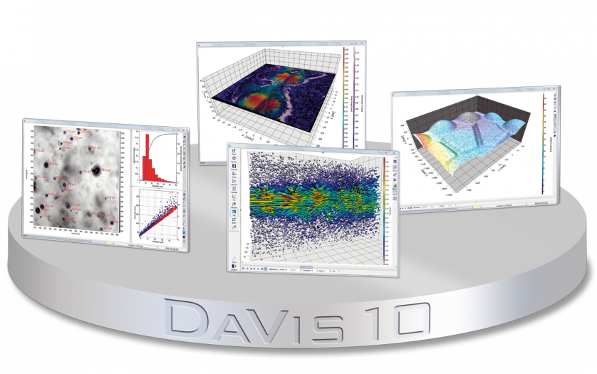
北京欧兰科技发展有限公司为您提供《3D拉格朗日粒子追踪测速》,该方案主要用于航空中速度矢量场检测,参考标准《暂无》,《3D拉格朗日粒子追踪测速》用到的仪器有Shake-the Box 高空间分辨体视粒子跟踪测速、LaVision DaVis 智能成像软件平台。
我要纠错


 咨询
咨询