ICP-AES系列学习8:Spectral Interferences: Types, Avoidance, and C

tzl75

2005/03/25

私聊

ICP光谱

8. Spectral Interferences: Types, Avoidance, and Correction

For your convenience, spectral interference topics have been broken into separate sections for both ICP-OES and ICP-MS users. However, the majority of this chapter is concerned with spectral interference correction for ICP-OES.

Types: ICP-OES
The types of spectral interferences most commonly encountered for ICP-OES are discussed in the Spectral Interferences section of our Reliable Measurements series. You may wish to review this information before continuing.

As noted in part 7 of this guide, the collection of spectra at different concentrations on all elements and lines available will save a lot of time in the line selection process.

Avoidance: ICP-OES
Several modern ICP instruments have the capability of avoiding the spectral interference by going to another line. Many instruments can make measurements simultaneously on several lines for 70+ elements in the same time it used to take to make a measurement on a single line/element combination. If you have the opportunity, I would strongly encourage the avoidance approach over attempting to make correction on a direct spectral overlap or wing overlap interference. Background corrections are another manner and can be routinely dealt with.

Correction: ICP-OES
Examples are provided below for background interference and spectral overlap.

Background Interference:
Background radiation is a potential source of error that requires correction. The source of the background radiation is from a combination of sources that cannot be easily controlled by the operator. Figure 8.1 shows the spectra for a highly concentrated Ca sample as compared to a nitric acid blank.

Figure 8.1:
Spectrum of 6% Ca solution vs. nitric acid blank

The background radiation intensity for the nitric acid blank is ~ 110,000 counts at 300 nm whereas the background radiation for the Ca containing solution is ~ 170,000 counts at the same wavelength. Although background radiation can be lowered somewhat by adjusting instrumental parameters, it cannot be eliminated and corrections are typically necessary. It can be seen that the highly concentrated Ca matrix contributes some to the background radiation but there are greater contributions from other sources independent of the sample matrix.

It can be argued that matrix-matched standards and samples will eliminate the need for background correction where the analyst only has to measure the peak intensity. It would follow that the precision of the measurement would be better (lower) and for some instruments the measurement time will be shorter. However, the problems with matrix matching are obvious and may offset any advantage gained when you don抰 make them.

The correction for background radiation is typically made by first selecting background points or regions and then a correction mode or algorithm. The 慳lgorithm?or 慶orrection mode?depends upon the curvature of the background, as is illustrated below.

Figure 8.2:
Flat background correction

Figure 8.2 shows a flat background where correction was made on both sides of the line. In this case the instrument allows for the selection of background regions thereby improving the accuracy of the estimated background radiation. If the instrument only allows for selection of background points then intensities are taken at set wavelengths, averaged and subtracted from the peak intensity. For flat backgrounds the distance of each point from the peak intensity is not important provided there is no interference from other lines in that vicinity. Figure 8.2 demonstrates that care was taken to avoid The Re line on the long wavelength side of the Zn 213.856 nm line and that a straight line that accurately determines the background intensity in the peak area is obtained.

Figure 8.3 shows a sloping but linear background. If the instrument only allows for selection of background points then intensities are taken at set wavelengths, averaged and subtracted from the peak intensity. Here, background points must be taken equal distance from the peak center in order to make an accurate correction. Again, a linear fit was used.

Figure 8.3:
Sloping background correction

Curved backgrounds are encountered when the analytical line is near a high intensity line, as is the case shown in Figure 8.4 below. In this case an algorithm estimating a curve (parabola) was used. For some instruments, depending upon design and software, this type of correction can be very difficult. This is a case where the 589.592 nm Na line would allow for the easier linear correction without loss in sensitivity.

Figure 8.4:
Curved background correction

Spectral Overlap:
For purposes of demonstration the interference of the As 228.812 nm line upon the Cd 228.802 nm lime will be used. In this example, the analysts is attempting to determine the feasibility of measuring Cd in the 0.05 to 100 礸/mL range with 100 礸/mL As present. The analyst would like to have both elements present in the calibrations samples as well as make accurate Cd determinations in unknown samples. The analyst would also like to estimate the detection limit for Cd under these conditions.

As discussed in part 7 of this guide, spectra collected at the time of the establishment of a given instrument in the laboratory can save significant time later. In this case, we will be using spectra collected just after the instrument was installed. It is true that the instrument has aged and it抯 performance characteristic may be different (better or worse), but the analyst can still call upon the aid of these data to gain some insight into the feasibility of making a given determination. Consequently, Figure 8.5 shows the spectra for solutions containing 0.1, 1.0 10 and 100 礸/mL Cd along with the spectrum of a 100 礸/mL As solution.

Figure 8.5:
Spectra for 100 礸/mL As and 0.1, 1.0, 10, and 100 礸/mL Cd

(Figure 8.5 - zoomed view)

精
该帖子已被管理者-西北狼设置为精华，下面是奖励记录：加5积分,加5声望

相关话题

+关注

私聊

第1楼2005/03/25

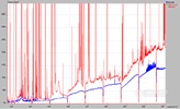
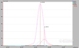
Table 8.1 contains intensity data collected from Figure 8.5. This table shows:
(A) the concentration of Cd;
(B) the relative concentration of As to Cd;
(C) the net intensity of the corresponding Cd concentration with no As present;
(D) the estimated standard deviation of measurement of Cd;
(E) the net intensity of 100 ppm As at the 228.802 nm wavelength;
(F) the estimated standard deviation for measurement of As;
(G) the estimated standard deviation of the combined signals for As at 100 ppm and Cd at the concentrations given;
(H) the uncorrected relative error for measuring Cd 228.802 nm with 100 ppm As present, and;
(I) the best-case relative errors for correcting the Cd intensity to account for 100 ppm As.

Table 8.1:
Estimated Errors of As on Cd 228.802 nm line

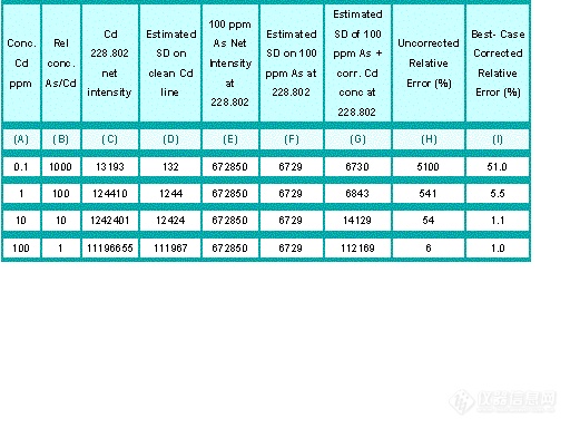
It was assumed that the precision (expressed above as standard deviation) of measuring the intensity of the As or Cd contributions at 228.802 nm is 1%. In addition, it was assumed that the best-case precision for making a correction is calculated using the following equation:

SDcorrection = [(SDCd I)2 + (SDAs I)2]1/2

where:

SDcorrection = standard deviation of the corrected Cd intensity;
SDCd I= standard deviation of the Cd intensity at 228.802 nm;
SDAs I = standard deviation of the As intensity at 228.802 nm
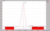
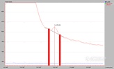
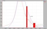
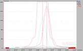
We can see from the above assumptions that a very optimistic view was taken in making this assessment. If we assume that a best-case detection limit for Cd at 228.802 nm in the presence of 100 ppm As would be 2 x SDcorrection, then the calculated detection limit is 0.1 ppm. In reality, the detection limit would be closer to .5 ppm. The detection limit for the Cd 228.802 nm line is 0.004 ppm (spectrally clean) showing roughly a 100-fold loss. Furthermore, the lower limit of quantitation has been increased form 0.04 ppm (10 x the DL) to somewhere between 1 and more realistically 5 ppm Cd. Figure 8.6 illustrates the situation with the spectra of 1 and 10ppm Cd solutions with and without 100 ppm As present.

Figure 8.6:
1 and 10 ppm Cd with and without 100 ppm As

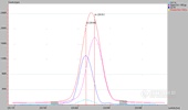
Correcting for the interference of As upon Cd would require that (1) the As concentration in the solution be measured and that (2) the analyst already have measured the counts/ppm As at the 228.802 nm line (sometimes called correction coefficient). This information allows for a correction by subtracting the calculated intensity contribution of As upon the 228.802 nm Cd line, thereby making the correction. This approach further assumes that slight changes in the instrumental operating parameters and conditions will influence both the analyte (Cd) and the interfering element (As) equally (i.e., an assumption many analysts are not willing to make).

The problems associated with direct spectral overlap make it difficult for the analyst to perform quantitative measurements. Each case should be reviewed. If a spectral correction is found to be necessary, the reader is advised to consult their operating manual where a defined procedure will be outlined using the instrument抯 software.

Types: ICP-MS
The types of spectral interferences most commonly encountered for ICP-MS are discussed in the Spectral Interferences section of our Reliable Measurements series. You may wish to review this information before continuing.

Avoidance: ICP-MS
The following are possible avoidance pathways:

The use of high resolution ICP-MS.

Matrix alteration through elimination ?for example, elimination of S, and halogen containing reagents such as Cl.

The use of reaction and or collision cells to destroy molecular interfering ions.

Cool plasma to reduce background interferences.

Separation of analyte(s) ?for example the use of chromatography or solvent extraction, etc.

The use of alternate ICP discharges such as He, mixed gas (He-Ar, N2-Ar, etc.).

Low-Pressure ICP discharges.

The above approaches are just examples of some of the approaches that have been taken to avoid interferences. For a given application, it is suggested that a literature search be performed in an attempt to benefit form the vast amount of research that has been conducted in this area. In addition, instrument manufacturers are constantly revising and updating their instrumentation and software in an attempt to take advantage of new technologies. Thus, consulting with the manufacturer may help when interferences are encountered.

The fact is that the mass spectra of elements are much less detailed than in optical emission spectroscopy. Most elements have fewer than seven isotopes and many have only one (monoisotopic). When interference is encountered, it may be possible to go to another isotope even if it is less abundant. The difficulty in obtaining low detection limits in ICP-MS with interference correction is a function of the relative signal intensities and measurement precision as illustrated above for ICP-OES. If a correction cannot be avoided, many analysts seek alternate techniques rather than run the risk of reporting unreliable data.